|
(continued...)
If the direct effects of CO2 are minimal and the future scenarios are relatively
warm, decreases in LAI could occur over very large forested areas, ranging up
to nearly 2/3 or more of the areas of boreal, temperate and tropical forests
(Table C-2). By contrast, if the direct effects
of CO2 are strong and scenarios are not too warm, then all forest vegetation
zones could experience increased biomass over as much as 2/3 or more of their
areas (Table C-3). More likely, the responses
will be intermediate with large regional contrasts, decreases in vegetation
density in some areas, increases in others. Even though these are equilibrium
simulations, a simulated decline in LAI generally implies a less favorable water
balance and a loss of vegetation density. These losses imply a process of loss
over some time period. We can only draw inferences about how rapidly such losses
would occur, based on the simulated amount of loss. The regions that could experience
declining LAI (Figure C-6, Figure
C-7, Figure C-8 and Figure
C-9), would exhibit spatial gradients in response from mild decline grading
into potentially catastrophic dieback. All reaches along the decline gradients
would experience drought stress, which could trigger other responses, such as
pest infestations and fire. Following disturbance by drought, infestation or
pests, new vegetation, either of the same or of a different type would grow,
but to a lower density.
Including both equilibrium and 'transient' scenarios, MAPSSwas run under four
different scenarios (not counting the sulfate scenario, HADSUL). These range
in global temperature increase (delta T) at the time of 2 x CO2 from 1.7 (HADGHG)
to 5.2�C (UKMO) (Annex B). In general, the areas of forest decline within individual
biomes (incorporating a direct CO2 effect) increase linearly with increasing
delta T in the temperate and boreal forests; while, the areas of increased forest
density decrease with increasing delta T. Tropical forests exhibit a similar
pattern across the three FAR scenarios, but under the cooler HADGHG scenario
show a large decline as simulated by MAPSS. By contrast, BIOME3, under the HADGHG
scenario, shows almost no change in tropical forest density. Interestingly,
adjacent tropical savannas increase in density in both ecological models under
the HADGHG scenario.
C.6.4. Equilibrium vs. "Transient" Scenarios and the Importance of Elevated
CO2
The newer climate scenarios (IPCC 1996, WG I, Section 6), extracted from transient
GCM simulations, are as a group quite different from the older, equilibrium
scenarios (IPCC 1990, WG I, Section 3), in terms of the simulated ecological
responses that these scenarios produce. All of the older scenarios produce large
regions showing LAI declines (especially in temperate to high latitudes), as
well as gains, even when the direct effects of CO2 are included (MAPSS simulations,
Figure C-6, OSU and UKMO scenarios not shown).
By contrast, under the newer scenarios, if a direct CO2 effect is assumed, then
there are very few regions with declines in LAI, as simulated by both MAPSS
and BIOME3 (Figures C-7, C-8);
rather, most of the world is simulated with an increased LAI. Actual increases
in LAI could be limited by nitrogen availability in some areas, although elevated
soil temperatures could increase decomposition, releasing more nitrogen (McGuire
et al., 1995; VEMAP Members, 1995). The first-order differences between the
older and newer scenarios are likely due to the smaller global temperature increases
in the newer climate scenarios, which came from GCMs that had not attained their
full equilibrium temperature changes.
C.6.5. Sulfate Aerosols
The incorporation of sulfate aerosols produced a cooling effect in the HADCM2SUL
run compared to the HADCM2GHG run, which lacked the sulfate forcing (GHG runs
are not shown). The vegetation response to the sulfate forcing is observable
in the model output from both MAPSS and BIOME3, but is relatively small compared
to the differences between the newer and older climate scenarios. The newer
scenarios produce widespread enhanced vegetation growth, even without the sulfate
effect, if direct CO2 effects are included and widespread decline if the CO2
effects are excluded. The presence of the sulfate-induced cooling produces a
much smaller amplitude effect on the vegetation than does the presence or absence
of the direct effects of elevated CO2 on water-use-efficiency.
C.6.6. Change in Annual Runoff
Changes in annual runoff (Figure C-10) were mapped
for all scenarios from both MAPSS and BIOME3. The changes in runoff are more
stable among the different climate scenarios than are the simulated changes
in LAI. The relative stability of simulated runoff change may reflect that runoff
is a passive drainage process; whereas, evapotranspiration is a biological process
and a function of the product of LAI and stomatal conductance. If stomatal conductance
is reduced, e.g., via a direct CO2 effect, LAI will compensate by increasing
and runoff will show little change (Neilson and Marks, 1994). Some of the obvious
differences between MAPSS and BIOME3 can be attributed to structural differences
in the models. BIOME3 calculates water balance daily, even though all inputs
are monthly; whereas, MAPSS calculates water balance monthly. This difference
alone could be causing the more extreme responsiveness of MAPSS, which shows
both larger runoff increases and larger losses in different regions. On the
other hand, MAPSS uses a 3-layer soil with roots only in the top two layers;
while BIOME3 uses a 2-layer soil with roots in both layers. The third layer
in MAPSS provides a consistent base flow and might explain why MAPSS produces
runoff in some drier regions, such as the western U.S., while BIOME3 does not.
The hydrology models in both MAPSS and BIOME3, although process-based, are considered
prototypes for eventual replacement by more elaborate models (see for example,
the PILPS model intercomparison study; Love and Henderson-Sellers, 1994).
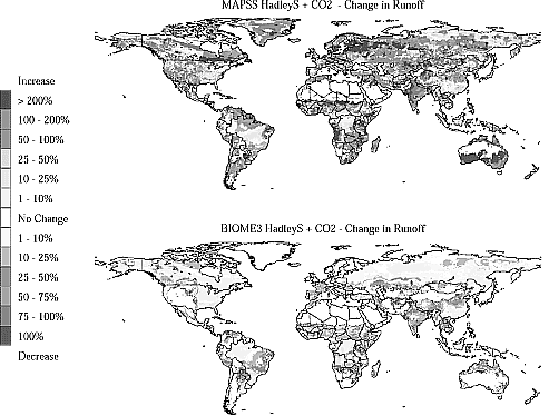 |
| Figure C-10: The potential change in annual runoff, as simulated
under the HADCM2SUL GCM experiment (Hadley Center, 2 x CO2 greenhouse gas
radiative forcing, extracted from transient simulation, plus sulfate aerosols),
by (a) MAPSS and (b) BIOME3. Both models have incorporated a direct, physiological
CO2 effect. This figure is a companion to Figures
C-4 and C-8. |
In general, MAPSS and BIOME3 produce similar regional patterns in the estimated
changes in runoff. Although the magnitude of the changes are different, there
are broad similarities in the sign of the change (but, clearly not in all regions).
The largest area of regional difference between the two models is in interior
Eurasia (Figure C-10).
Runoff generally increases in the Tundra, due to higher temperatures, more
precipitation and more melting (Tables C-4, C-5).
It decreases in the Taiga/Tundra due to encroachment of high-density boreal
forest into low density vegetation (hence, higher transpiration). Runoff results
are varied in the temperate forests, but Temperate Mixed forests tend to present
a higher likelihood of reduced runoff over large areas (range 51% to 88% of
the area under all scenarios) than of increased runoff (range 11% to 47% of
the area under all scenarios, Tables C-4, C-5).
Even the most benign scenarios indicate a minimum of 51% of the area of the
world's temperate evergreen forests could experience a runoff decline; whereas,
a maximum of 47% of the area would experience increased runoff. Temperate Evergreen
Forests exhibit a greater likelihood of increased runoff over large areas (range
29% to 87% of the area under all scenarios) than decreased runoff (range 11%
to 68%), but the overlap in these increase and decrease ranges indicates the
degree of uncertainty in the simulations. However, much of the increased runoff
in the Temperate Evergreen forested areas is due to increased winter runoff,
which is not necessarily available for use by ecosystems, irrigation or domestic
purposes. Runoff from tropical forest areas could either increase or decrease
over large areas, depending largely on the importance of the direct CO2 effects.
Runoff from drier vegetation types is regionally variable and exhibits both
increases and decreases, depending on the direct CO2 effects and regional rainfall
patterns.
|