|
3.7.3. Tools Capable of Addressing Interactions
Most climate scenarios for impact assessments were developed by using outputs
from AOGCMs (Hulme and Brown, 1998). Often these results are scaled toward the
desired emission levels with simple climate models (Hulme et al., 1995;
Harvey et al., 1997; see Section 3.8.3). In
this simple approach, most interactions are neglected.
The only models that can be used to develop more consistent scenarios that
incorporate most of the important interactions are IAMs (see Section
3.3.2.3). IAMs have been developed with different levels of complexity,
from extremely simple to highly complex (Harvey et al., 1997). Different
interactions are included, although no single model provides a fully comprehensive
treatment. The models are most commonly used for emission scenario development
and mitigation policy assessment (Schimel et al., 1997a; Alcamo et
al., 1998a; Pepper et al., 1998). All simulate a causal chain (e.g.,
human activities, emissions, climate change, sea-level rise, and other impacts).
Emissions, climate change, impact, and mitigation scenarios derived from these
models have been published (Schimel et al., 1997a; Leemans et al.,
1998; Pepper et al., 1998) and collected in several databases (Alcamo
et al., 1995; Nakicenovic et al., 2000). Unfortunately, it is
not always clear which interactions are explicitly included in individual IAMs.
This reduces the comparability of individual IAM-derived scenarios and thus
their utility.
Depending on assumed interactions during scenario development, a wide range
of estimates of climate change and its impacts is possible (see Table
3-7). However, within this range certain responses are more likely than
others. To define appropriate and realistic levels of interactions, expert judgment
and sensitivity experiments with models could be very valuable (van der Sluijs,
1997). Innovative, objective, and systematic approaches have to be developed
to evaluate underlying scenario assumptions and to validate the scenario results.
This is still an immature area of scenario development.
3.7.4. Problems of Compatibility between Scenarios
One difficulty faced by authors in attempting to summarize and synthesize the
results of impact studies for previous IPCC assessments (i.e., IPCC, 1996b,
1998) has been a lack of consistency in projections. Different climate projections
have been adopted in different studies, in different regions (or within the
same region), and in different sectors. Moreover, even where the same climate
projections are assumed, they might not be applied in the same way in different
impact studies. Finally, some studies also are inconsistent in their methods
of projecting changes in climate alongside concurrent changes in related socioeconomic
and environmental conditions.
For example, GHG concentrations often are transformed into CO2-equivalent
concentrations to determine radiative forcing levels and climate change. The
GCM community often presents climate change simulations as "doubled CO2"
anomalies. Depending on the scenario, however, 5-40% of the forcing is
caused by non-CO2 GHGs (30% in 1990). The doubled-CO2
scenarios often are interpreted as CO2 only (e.g., Cramer et al.,
1997); others add an explicit distinction between CO2 and non-CO2
gases (e.g., Downing et al., 1999). In determining the impacts of direct
CO2 effects and climate change, this can easily lead to inconsistencies.
Similar discrepancies exist for other types of interactions.
Finally, it is a significant challenge to integrate climate or sea-level rise
scenarios, with a time horizon of decades to hundreds of years, with nonclimatic
scenarios of social, economic, and technological systems that can change rapidly
over a time scale of years. For instance, it is difficult to devise credible
socioeconomic scenarios that extend beyond the lifetime of current infrastructure
and institutions. Moreover, social/economic actors who need to be involved in
the scenario development process (e.g., business, governments) often find long
time horizons difficult to contemplate. Box 3-2
illustrates a recent example of an attempt to harmonize climate change, sea
level, atmospheric composition, and socioeconomic scenarios in a multi-sectoral
global impact assessment.
|

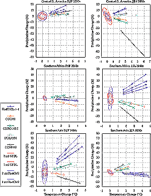
Figure 3-2: Scaled outputs of mean December-February
(left) and June-August (right) temperature and precipitation change
by the 2050s relative to 1961-1990 over land grid boxes representing
Central North America (top), Southern Africa (middle), and Southern
Asia (bottom) from eight simulations with five AOGCMs (experiments b,
c, e, h, and a four-member ensemble from t; see Table
3-5). Simulations assume forcing by greenhouse gases but not aerosols,
and are standardized according to the climate sensitivity of each AOGCM.
Lines connect four points for each simulation, all in the same order
from the origin: B1-low, B2-mid, A1-mid, A2-high. Each point represents
the standardized regional changes in climate from the AOGCM, linearly
scaled according to the global warming estimated with a simple climate
model for one of four preliminary SRES marker emissions scenarios (B1,
B2, A1, and A2) and a value of the climate sensitivity (low = 1.5°C;
mid = 2.5°C, and high = 4.5°C). Also plotted are ±1 and
±2 standard deviation ellipses from the 1400-year HadCM2 and
1000-year GFDL unforced simulations, which are used to indicate natural
multi-decadal variability and are orientated according to the correlation
between modeled 30-year mean temperature and precipitation. Results
from two other AOGCMs did not extend to the 2050s (Carter et al., 2000).
|
|