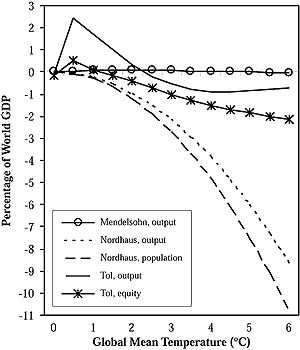
Figure 19-4: Monetary impacts as a function of level of climate change (measured as percentage of global GDP). Although there is confidence that higher magnitudes and rates of increase in global mean temperature will lead to increasing damages, there is uncertainty about whether aggregate damages are positive or negative at relatively low increases in global mean temperature.

One of the main challenges of impact assessments is to move from the static analysis of certain benchmarks to a dynamic representation of impacts as a function of shifting climatic parameters, adaptation measures, and exogenous trends such as economic and population growth. Little progress has been made in this respect, and our understanding of the time path that aggregate impacts will follow under different warming and development scenarios still is extremely limited. Among the few explicitly dynamic analyses are Sohngen and Mendelsohn (1999) and Yohe et al. (1996).

Some information about impacts over time is available for individual sectors. Scenarios derived from IAMs can provide comprehensive emissions, concentrations, and climate change estimates that can be linked to impact models. Table 19-5 summarizes estimates of global ecosystem impacts that were derived from such a model (IMAGE 2.1—Leemans et al., 1998; Swart et al., 1998). The metric used is percentage change. The example illustrates the clearly nonlinear dynamics of nonmarket impacts with different pathways for positive (escalating) and negative (saturating) impacts. The impact levels in this model evolve gradually, and there are impacts even at low levels of climate change. Although this finding is consistent with observed change (see Section 19.2), it is sensitive to the choice of metric. White et al. (1999), for example, found that carbon storage in terrestrial vegetation would expand under moderate warming because increases in productivity are enough to offset reductions elsewhere. They show that as higher GHG concentrations and magnitudes of climate change are reached, carbon storage eventually will decline.

Little is known about the shape of the aggregate impact function. Dynamic functions remain highly speculative at this point because the underlying models provide only a very rough reflection of real-world complexities. Figure 19-4 provides examples from three studies. Although some analysts still work with relatively smooth impact functions (e.g., Nordhaus and Boyer, 2000), there is growing recognition (e.g., Mendelsohn and Schlesinger, 1997; Tol, 2001c) that climate change dynamics in fact might be more complex and may not follow a monotonic path. Generic patterns that are emerging include the following:

• Moderate climate change may have positive and negative effects, with most positive effects occurring in the market sector of developed countries. For higher levels of warming, impacts are likely to become predominantly negative. However, the overall pattern is complex, estimates remain uncertain, and the possibility of highly deleterious outcomes cannot be excluded (medium confidence).
  
• Impacts in different sectors may unfold along different paths. Coastal impacts, for example, are expected to grow continuously over time, more or less in proportion to the rise in sea level. The prospects for agriculture, by contrast, are more complex. Whereas some models predict aggregate damages already for moderate warming, many studies suggest that under some (but not all) scenarios the impact curve might be hump-shaped, with short-term (aggregate) benefits under modest climate change turning into losses under more substantial change (e.g., Mendelsohn and Schlesinger, 1997) (low confidence).

Aggregating intertemporal impacts into a single indicator is extremely difficult, perhaps elusive. The marginal damages caused by 1 t of CO₂ emissions in the near future were estimated in the SAR at US$5-125 t-1 C. Most estimates are in the lower part of that range; higher estimates occur only through the combination of high vulnerability with a low discount rate (see Pearce et al., 1996). Plambeck and Hope (1996), Eyre et al. (1997), and Tol (1999a) have since reassessed the marginal costs of GHG emissions. Performing extensive sensitivity and uncertainty analyses, they arrive at essentially the same range of numbers as Pearce et al. (1996). In the complex dynamics that determine marginal damage costs, the more optimistic estimates of market damages used in recent studies are balanced out by other factors such as higher nonmarket impacts and a better capture of uncertainties. Overall, the SAR assessment still is a good reflection of our understanding of marginal damage costs; our confidence in marginal damage numbers remains very low.

Table 19-5: Aggregate impact of climate change on ecosystems (Swart et al., 1998). See also list of caveats in Section 19.4.1.
	Scenario
Impact Indicator	0.5°C	1.0°C	1.5°C	2.0°C	2.5°C	3.0°C
Temperate cereals, area experiencing
- Yield decreasea	12	16	18	20	20	22
- Yield increasea	2	3	4	8	12	15
Maize, land area experiencing
- Yield decreasea	13	18	22	26	29	33
- Yield increasea	2	4	6	9	13	17
Change in natural vegetationb	11	19	26	32	37	43
Endangered nature reservesc	9	17	24	32	37	42
a Yield decrease and increase are percentage area with at least 10% change in potential rainfed yield. Reference area is current crop area. b Change in natural vegetation is percentage of land area that shifts from one vegetation type to another. Reference area is global land area. c Endangered nature reserves are percentage of reserves, where original vegetation disappears, so that conservation objectives cannot be met. Reference is total reserve number.

IPCC Homepage