|
8.4.3 Economywide Impact of CO2 Stabilization in the Post-SRES
Scenarios
The economy-wide impact of stabilizing atmospheric CO2 concentrations
was assessed based on 42 post-SRES stabilization scenarios developed using the
AIM, ASF, MARIA, MiniCAM, MESSAGE, and World SCAN models. These scenarios were
developed by applying various mitigation policies and measures to the six illustrative
scenarios (baselines) presented in the Special Report on Emission Scenarios
(SRES).
|

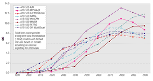
Figure 8.16: Reductions in carbon emissions for
the SRES A1B 550 case.
|

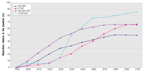
Figure 8.17: Time path of emissions reductions.
|
The economy-wide impact of CO2 stabilization was assessed on the
basis of the difference in GDP in baseline scenarios and corresponding stabilization
cases in a given year. This difference is expressed in percent (reflecting a
relative GDP loss) and is positive when GDP in a baseline scenario is larger
than in a stabilization case and is negative when GDP in a stabilization scenario
is larger. Such an approach to measuring effects of stabilization was selected
since it better reflects the societal burden of emission stabilization than
absolute changes in GDP. For example, a 1% reduction in the 2100 GDP of the
SRES A1 world is equal to about US$5.5 trillion and is larger in absolute terms
than a 2% or US$5.0 trillion reduction in the 2100 GDP of the poor A2 world.
Nonetheless, the relative level of effort in the latter case would be much greater.
It should be also emphasized here that the GDP reduction itself represents a
very crude indicator of economic consequences of the CO2 stabilization.
For example, most of the stabilization scenarios reviewed here have not rigorously
accounted for the economic effects of introducing new low-emission technologies,
new revenue rising instruments or adequate inter-regional financial and technology
transfers, all elements which contribute to lower the costs as explained in
the rest of the chapter.
|

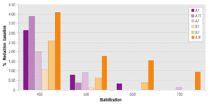
Figure 8.18: Global average GDP reduction in 2050 for alternative
stabilization targets and six SRES reference scenarios.
|
The average GDP reduction in most of the stabilization
scenarios reviewed here is under 3% of the baseline value (the maximum reduction
across all the stabilization scenarios reached 6.1% in a given year). At the
same time, some scenarios (especially in the A1T group) showed an increase in
GDP compared to the baseline due to apparent positive economic feedbacks of
technology development and transfer. The GDP reduction (averaged across storylines
and stabilization levels) is lowest in 2020 (0.99%), reaches a maximum in 2050
(1.45%) and declines by 2100 (1.30%). However, in the scenario groups with the
highest baseline emissions (A2 and A1FI), the size of the GDP reduction increases
throughout the modelling period.
Due to their relatively small scale when compared to absolute GDP levels, GDP
reductions in the post-SRES stabilization scenarios do not lead to significant
declines in GDP growth rates over this century. For example, the annual 1990-2100
GDP growth rate across all the stabilization scenarios was reduced on average
by only 0.003% per year, with a maximum reduction reaching 0.06% per year.
Figure 8.18 shows the relationship between the relative
GDP reduction, the scenario group, and the stabilization level in 2050. The
reduction in GDP tends to increase with the stringency of the stabilization
target. But the costs are very sensitive to the choice of baseline scenario.
The maximum relative reduction occurs in the A1FI scenario group, followed by
the other A1 scenario groups and the A2 group, while the minimum reduction occurs
in the B1 group20
. By 2100, the situation slightly changes with GDP reductions in the A2 scenario
group becoming relatively more pronounced.
|

Figure 8.19: Average GDP and CO2 reductions in 550ppmv
stabilization scenarios: year 2050 (labels identify different scenario
groups).
|
Differences in relative GDP reductions in different scenario groups are explained
by the magnitude of corresponding CO2 emission reductions needed
to achieve a particular stabilization level. The emission reduction is apparently
the largest in the A1FI scenario group, which is also associated with the
largest GDP loss (Figure 8.19). Meanwhile, the smallest
relative GDP loss occurs in the A1T and B1 groups, which have low baseline
emissions and accordingly require the smallest reductions to reach the CO2
stabilization.
Regional GDP reduction patterns in the post-SRES stabilization scenarios
are also generally explained by corresponding required reductions in CO2
emissions, which are determined by baseline emissions, the stabilization levels,
assumptions about emissions trading mechanisms and about the relative contribution
of regions to global CO2 emissions; reduction and associated financial
and technology transfer. In most of the baseline (SRES) scenarios starting
from 2020, absolute CO2 emissions in developing (non-Annex I) regions
remain larger for the rest of the 21st century than in the industrialized
(Annex I) regions.
|