2.10 Global Warming Potentials and Other Metrics for Comparing Different Emissions

2.10.1 Definition of an Emission Metric and the Global Warming Potential

Multi-component abatement strategies to limit anthropogenic climate change need a framework and numerical values for the trade-off between emissions of different forcing agents. Global Warming Potentials or other emission metrics provide a tool that can be used to implement comprehensive and cost-effective policies (Article 3 of the UNFCCC) in a decentralised manner so that multi-gas emitters (nations, industries) can compose mitigation measures, according to a specified emission constraint, by allowing for substitution between different climate agents. The metric formulation will differ depending on whether a long-term climate change constraint has been set (e.g., Manne and Richels, 2001) or no specific long-term constraint has been agreed upon (as in the Kyoto Protocol). Either metric formulation requires knowledge of the contribution to climate change from emissions of various components over time. The metrics assessed in this report are purely physically based. However, it should be noted that many economists have argued that emission metrics need also to account for the economic dimensions of the problem they are intended to address (e.g., Bradford, 2001; Manne and Richels, 2001; Godal, 2003; O’Neill, 2003). Substitution of gases within an international climate policy with a long-term target that includes economic factors is discussed in Chapter 3 of IPCC WGIII AR4. Metrics based on this approach will not be discussed in this report.

A very general formulation of an emission metric is given by (e.g., Kandlikar, 1996):

AM_i = ∫^∞₀ [(I(DC _{(r + i)} (t)) – I (DC_r (t))) x g(t)]dt

where I(∆C_i(t)) is a function describing the impact (damage and benefit) of change in climate (∆C) at time t. The expression g(t) is a weighting function over time (e.g., g(t) = e^–kt is a simple discounting giving short-term impacts more weight) (Heal, 1997; Nordhaus, 1997). The subscript r refers to a baseline emission path. For two emission perturbations i and j the absolute metric values AM_i and AM_j can be calculated to provide a quantitative comparison of the two emission scenarios. In the special case where the emission scenarios consist of only one component (as for the assumed pulse emissions in the definition of GWP), the ratio between AM_i and AM_j can be interpreted as a relative emission index for component i versus a reference component j (such as CO₂ in the case of GWP).

There are several problematic issues related to defining a metric based on the general formulation given above (Fuglestvedt et al., 2003). A major problem is to define appropriate impact functions, although there have been some initial attempts to do this for a range of possible climate impacts (Hammitt et al., 1996; Tol, 2002; den Elzen et al., 2005). Given that impact functions can be defined, AM calculations would require regionally resolved climate change data (temperature, precipitation, winds, etc.) that would have to be based on GCM results with their inherent uncertainties (Shine et al., 2005a). Other problematic issues include the definition of the temporal weighting function g(t) and the baseline emission scenarios.

Due to these difficulties, the simpler and purely physical GWP index, based on the time-integrated global mean RF of a pulse emission of 1 kg of some compound (i) relative to that of 1 kg of the reference gas CO₂, was developed (IPCC, 1990) and adopted for use in the Kyoto Protocol. The GWP of component i is defined by

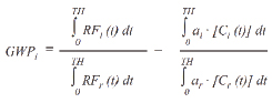
where TH is the time horizon, RF_i is the global mean RF of component i, a_i is the RF per unit mass increase in atmospheric abundance of component i (radiative efficiency), [C_i(t)] is the time-dependent abundance of i, and the corresponding quantities for the reference gas (r) in the denominator. The numerator and denominator are called the absolute global warming potential (AGWP) of i and r respectively. All GWPs given in this report use CO₂ as the reference gas. The simplifications made to derive the standard GWP index include (1) setting g(t) = 1 (i.e., no discounting) up until the time horizon (TH) and then g(t) = 0 thereafter, (2) choosing a 1-kg pulse emission, (3) defining the impact function, I(∆C), to be the global mean RF, (4) assuming that the climate response is equal for all RF mechanisms and (5) evaluating the impact relative to a baseline equal to current concentrations (i.e., setting I(∆C_r(t)) = 0). The criticisms of the GWP metric have focused on all of these simplifications (e.g., O’Neill, 2000; Smith and Wigley, 2000; Bradford, 2001; Godal, 2003). However, as long as there is no consensus on which impact function (I(∆C)) and temporal weighting functions to use (both involve value judgements), it is difficult to assess the implications of the simplifications objectively (O’Neill, 2000; Fuglestvedt et al., 2003).

The adequacy of the GWP concept has been widely debated since its introduction (O’Neill, 2000; Fuglestvedt et al., 2003). By its definition, two sets of emissions that are equal in terms of their total GWP-weighted emissions will not be equivalent in terms of the temporal evolution of climate response (Fuglestvedt et al., 2000; Smith and Wigley, 2000). Using a 100-year time horizon as in the Kyoto Protocol, the effect of current emissions reductions (e.g., during the first commitment period under the Kyoto Protocol) that contain a significant fraction of short-lived species (e.g., CH₄) will give less temperature reductions towards the end of the time horizon, compared to reductions in CO₂ emissions only. Global Warming Potentials can really only be expected to produce identical changes in one measure of climate change – integrated temperature change following emissions impulses – and only under a particular set of assumptions (O’Neill, 2000). The Global Temperature Potential (GTP) metric (see Section 2.10.4.2) provides an alternative approach by comparing global mean temperature change at the end of a given time horizon. Compared to the GWP, the GTP gives equivalent climate response at a chosen time, while putting much less emphasis on near-term climate fluctuations caused by emissions of short-lived species (e.g., CH₄). However, as long as it has not been determined, neither scientifically, economically nor politically, what the proper time horizon for evaluating ‘dangerous anthropogenic interference in the climate system’ should be, the lack of temporal equivalence does not invalidate the GWP concept or provide guidance as to how to replace it. Although it has several known shortcomings, a multi-gas strategy using GWPs is very likely to have advantages over a CO₂-only strategy (O’Neill, 2003). Thus, GWPs remain the recommended metric to compare future climate impacts of emissions of long-lived climate gases.

Globally averaged GWPs have been calculated for short-lived species, for example, ozone precursors and absorbing aerosols (Fuglestvedt et al., 1999; Derwent et al., 2001; Collins et al., 2002; Stevenson et al., 2004; Berntsen et al., 2005; Bond and Sun, 2005). There might be substantial co-benefits realised in mitigation actions involving short-lived species affecting climate and air pollutants (Hansen and Sato, 2004); however, the effectiveness of the inclusion of short-lived forcing agents in international agreements is not clear (Rypdal et al., 2005). To assess the possible climate impacts of short-lived species and compare those with the impacts of the LLGHGs, a metric is needed. However, there are serious limitations to the use of global mean GWPs for this purpose. While the GWPs of the LLGHGs do not depend on location and time of emissions, the GWPs for short-lived species will be regionally and temporally dependent. The different response of precipitation to an aerosol RF compared to a LLGHG RF also suggests that the GWP concept may be too simplistic when applied to aerosols.