3.2.1.4 The use of MER in economic and emissions scenarios modelling
The uses of MER-based economic projections in SRES have recently been criticized (Castles and Henderson, 2003a, 2003b; Henderson, 2005). The vast majority of scenarios published in the literature use MER-based economic projections. Some exceptions exist, for example, MESSAGE in SRES, and more recent scenarios using the MERGE model (Manne and Richels, 2003), along with shorter term scenarios to 2030, including the G-Cubed model (McKibbin et al., 2004a, 2004b), the International Energy Outlook (USDOE, 2004), the IEA World Energy Outlook (IEA, 2004) and the POLES model used by the European Commission (2003). The main criticism of the MER-based models is that GDP data for world regions are not corrected with respect to purchasing power parities (PPP) in most of the model runs. The implied consequence is that the economic activity levels in non-OECD countries generally appear to be lower than they actually are when measured in PPP units. In addition, the high growth SRES scenarios (A1 and B1 families) assume that regions tend to conditionally converge in terms of relative per-person income across regions (see Section 3.1.4). According to the critics, the use of MER, together with the assumption of conditional convergence, lead to overstated economic growth in the poorer regions and excessive growth in energy demand and emission levels.
A team of SRES researchers responded to this criticism, indicating that the use of MER or PPP data does not in itself lead to different emission projections outside the range of the literature. In addition, they stated that the use of PPP data in most scenarios models was (and still is) infeasible, due to lack of required data in PPP terms, for example price elasticities and social accounting matrices (Nakicenovic et al., 2003; Grübler et al., 2004). A growing number of other researchers have also indicated different opinions on this issue or explored it in a more quantitative sense (e.g. Dixon and Rimmer, 2005; Nordhaus, 2006b; Manne and Richels, 2003; McKibbin et al., 2004a, 2004b; Holtsmark and Alfsen, 2004a, 2004b; Van Vuuren and Alfsen, 2006).
There are at least three strands to this debate. The first is whether economic projections based on MER are appropriate, and thus whether the economic growth rates reported in the SRES and other MER-based scenarios are reasonable and robust. The second is whether the choice of the exchange rate matters when it comes to emission scenarios. The third is whether it is possible, or practical, to develop robust scenarios given the sparseness of relevant and required PPP data. While the GDP data are available in PPP, other economic scenario characteristics, such as capital and operational cost of energy facilities, are usually available either in domestic currencies or MER. Full model calibration in PPP for regional and global models is still difficult due to the lack of underlying data. This could be one of the reasons why a vast majority of long-term emissions scenarios continues to be calibrated in MER.
On the question of whether PPP or MER should be employed in economic scenarios, the general recommendations are to use PPP where practical. This is certainly necessary when comparisons of income levels across regions are of concern. On the other hand, models that analyse international trade and include trade as part of their economic projections, are better served by MER data given that trade takes place between countries in actual market prices. Thus, the choice of conversion factor depends on the type of analysis or comparison being undertaken.
For principle and practical reasons, Nordhaus (2005) recommends that economic growth scenarios should be constructed by using regional or national accounting figures (including growth rates) for each region, but using PPP exchange rates for aggregating regions and updating over time by use of a superlative price index. In contrast, Timmer (2005) actually prefers the use of MER data in long-term modelling, as such data are more readily available, and many international relations within the model are based on MER. Others (e.g. Van Vuuren and Alfsen, 2006) also argue that the use of MER data in long-term modelling is often preferable, given that model parameters are usually estimated on MER data and international trade within the models is based on MER. The real economic consequences of the choice of conversion rates will obviously depend on how the scenarios are constructed, as well as on the type of model used for quantifying the scenarios. In some of the short-term scenarios (with a horizon to 2030) a bottom-up approach is taken where assumptions about productivity growth and investment/saving decisions are the main drivers of growth in the models (e.g. McKibbin et al., 2004a, 2004b). In long-term scenario models, a top-down approach is more commonly used where the actual growth rates are prescribed more directly, based on convergence or other assumptions about long-term growth potentials.
When it comes to emission projections, it is important to note that in a fully disaggregated (by country) multi-sector economic model of the global economy, aggregate index numbers play no role and the choice between PPP and MER conversion of income levels does not arise. However, in an aggregated model with consistent specifications (i.e. where model parameter estimation and model calibrations are all carried out based on consistent use of conversion factors), the effects of the choice of conversion measure on emissions should approximately cancel out. The reason can be illustrated by using the Kaya identity, which decomposes the emissions as follows:
GHG = Population x GDP per person x Emissions per GDP
or:
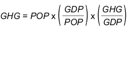
where GHG stands for greenhouse gas emissions, GDP stands for economic output, and POP stands for population size.
Given this relationship, emission scenarios can be represented, explicitly based on estimates of population development, economic growth, and development of emission intensity.
Population is often projected to grow along a pre-described (exogenous) path, while economic activity and emission intensities are projected based on differing assumptions from scenario to scenario. The economic growth path can be based on historical growth rates, convergence assumptions, or on fundamental growth factors, such as saving and investment behaviour, productivity changes, etc. Similarly, future emission intensities can be projected based on historical experience, economic factors, such as labour productivity or other key factors determining structural changes in an economy, or technological development. The numerical expression of GDP clearly depends on conversion measures; thus GDP expressed in PPP will deviate from GDP expressed in MER, particularly for developing countries. However, when it comes to calculating emissions (or other physical measures such as energy), the Kaya identity shows that the choice between MER-based or PPP-based representations of GDP will not matter, since emission intensity will change (in a compensating manner) when the GDP numbers change. While using PPP values necessitates using lower economic growth rates for developing countries under the convergence assumption, it is also necessary to adjust the relationship between income and demand for energy with lower economic growth, leading to slower improvements in energy intensities. Thus, if a consistent set of metrics is employed, the choice of metric should not appreciably affect the final emission level.
In their modelling work, Manne and Richels (2003) and McKibbin et al. (2004a, 2004b) find some differences in emission levels between using PPP-based and MER-based estimates. Analysis of their work indicates that these results critically depend on, among other things, the combination of convergence assumptions and the mathematical approximation used between MER-GDP and PPP-GDP. In the Manne and Richels work for instance, autonomous efficiency improvement (AEI) is determined as a percentage of economic growth and estimated on the basis of MER data. In going from MER to PPP, the economic growth rate declines as expected, leading to a decline in the autonomous efficiency improvement. However, it is not clear whether it is realistic not to change the AEI rate when changing conversion measure. On the other hand, Holtsmark and Alfsen (2004a, 2004b), showed that in their simple model consistent replacement of the metric (PPP for MER) – for income levels as well as for underlying technology relationships – leads to a full cancellation of the impact of choice of metric on projected emission levels.
To summarize: available evidence indicates that the differences between projected emissions using MER exchange rates and PPP exchange rates are small in comparison to the uncertainties represented by the range of scenarios and the likely impacts of other parameters and assumptions made in developing scenarios, for example, technological change. However, the debate clearly shows the need for modellers to be more transparent in explaining conversion factors, as well as taking care in determining exogenous factors used for their economic and emission scenarios.
Box 3.1 Market Exchange Rates and Purchasing Power Parity
To aggregate or compare economic output from various countries, GDP data must be converted into a common unit. This conversion can be based on observed market exchange (MER) rates or purchasing power parity (PPP) rates where, in the latter, a correction is made for differences in price levels between countries. The PPP approach is considered to be the better alternative if data is used for welfare or income comparisons across countries or regions. Market exchange rates usually undervalue the purchasing power of currencies in developing countries, see Figure 3.4.
Clearly, deriving PPP exchange rates requires analysis of a relatively large amount of data. Hence, methods have been devised to derive PPP rates for new years on the basis of price indices. Unfortunately, there is currently no single method or price index favoured for doing this, resulting in different sets of PPP rates (e.g. from the OECD, Eurostat, World Bank and Penn World Tables) although the differences tend to be small.