8.3. Structural and Technological Change
|

(click to enlarge)
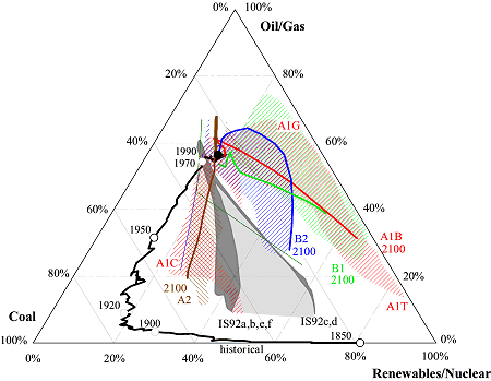
Figure TS-4: Global primary
energy structure, shares (%) of oil and gas, coal, and non-fossil (zero-carbon)
energy sources - historical development from 1850 to 1990 and in SRES
scenarios. Each corner of the triangle corresponds to a hypothetical
situation in which all primary energy is supplied by a single source
- oil and gas on the top, coal to the left, and non-fossil sources (renewables
and nuclear) to the right. Constant market shares of these energies
are denoted by their respective isoshare lines. Historical data from
1850 to 1990 are based on Nakicenovic et al. (1998). For 1990 to 2100,
alternative trajectories show the changes in the energy systems structures
across SRES scenarios. They are grouped by shaded areas for the scenario
families A1B, A2, B1, and B2 with respective markers shown as lines.
In addition, the four scenario groups within the A1 family A1B, A1C,
A1G, and A1T, which explore different technological developments in
the energy systems, are shaded individually. In the SPM, A1C and A1G
are combined into one fossil-intensive group A1FI. For comparison the
IS92 scenario series are also shown, clustering along two trajectories
(IS92c,d and IS92a,b,e,f). For model results that do not include non-commercial
energies, the corresponding estimates from the emulations of the various
marker scenarios by the MESSAGE model were added to the original model
outputs.
|
In this brief summary of the SRES scenarios, structural and technological changes
are illustrated by using energy and land use as examples. These examples are
characteristic for the driving forces of emissions because the energy system
and land use are the major sources of GHG and sulfur emission.
Chapter 4 gives a more detailed treatment of the full
range of emissions driving forces across the SRES scenarios.
Figure TS-4 illustrates that the change of world
primary energy structure diverges over time. It shows the contributions of individual
primary energy sources - the percentage supplied by coal, that by oil and gas,
and that by all non-fossil sources taken together (for simplicity of presentation
and because not all models distinguish between renewables and nuclear energy).
Each corner of the triangle corresponds to a hypothetical situation in which
all primary energy is supplied by a single source - oil and gas at the top,
coal to the left, and non-fossil sources (renewables and nuclear) to the right.
Historically, the primary energy structure has evolved clockwise according to
the two "grand transitions" (discussed in Chapter 3) that
are shown by the two segments of the "thick black" curve. From 1850 to 1920
the first transition can be characterized as the substitution of traditional
(non-fossil) energy sources by coal. The share of coal increased from 20% to
about 70%, while the share of non-fossils declined from 80% to about 20%. The
second transition, from 1920 to 1990, can be characterized as the replacement
of coal by oil and gas (while the share of non-fossils remained essentially
constant). The share of oil and gas increased to about 50% and the share of
coal declined to about 30%.
Figure TS-4 gives an overview of the divergent
evolution of global primary energy structures between 1990 and 2100, regrouped
into their respective scenario families and four A1 scenarios groups (three
in the SPM) that explore different technological developments in the energy
systems. The SRES scenarios cover a wider range of energy structures than the
previous IS92 scenario series, which reflects advances in knowledge on the uncertainty
ranges of future fossil resource availability and technological change.
In a clockwise direction, A1B, A1T, and B1 scenario groups map the structural
transitions toward higher shares of non-fossil energy in the future, which almost
closes the historical "loop" that started in 1850. The B2 scenarios indicate
a more "moderate" direction of change with about half of the energy coming from
non-fossil sources and the other half shared by coal on one side and oil and
gas on the other. Finally, the A2 scenario group marks a stark transition back
to coal. Shares of oil and gas decline while non-fossils increase moderately.
What is perhaps more significant than the diverging developments in these three
marker scenarios is that the whole set of 40 scenarios covers virtually all
possible directions of change, from high shares of oil and gas to high shares
of coal and non-fossils. In particular, the A1 scenario family covers basically
the same range of structural change as all the other scenarios together. In
contrast, the IS92 scenarios cluster into two groups, one of which contains
IS92c and IS92d and the other the four others. In all of these the share of
oil and gas declines, and the main structural change occurs between coal on
the one hand and non-fossils on the other. This divergent nature in the structural
change of the energy system and in the underlying technological base of the
SRES results in a wide span of future GHG and sulfur emissions.

(click to enlarge)
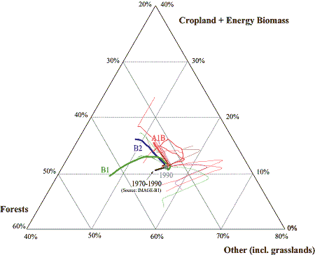
Figure TS-5: Global land-use patterns,
shares (%) of croplands and energy biomass, forests, and other categories
including grasslands - historical development from 1970 to 1990 (based
on B1-IMAGE) and in SRES scenarios. As for the energy triangle in Figure
6-3, each corner corresponds to a hypothetical situation in which land
use is dedicated to a much greater extent than today to one category
- 60% to cropland and energy biomass at the top, 80% to forests to the
left, and 80% to other categories (including grasslands) to the right.
Constant shares in total land area of cropland and energy biomass, forests,
and other categories are denoted by their respective isoshare lines.
For 1990 to 2100, alternative trajectories are shown for the SRES scenarios.
The three marker scenarios A1B, B1, and B2 are shown as thick colored
lines, and other SRES scenarios as thin colored lines. The ASF model
used to develop the A2 marker scenario projects only land-use change
related GHG emissions. Comparable data on land cover changes are therefore
not available.The trajectories appear to be largely model specific and
illustrate the different views and interpretations of future land-use
patterns across the scenarios (e.g. the scenario trajectories on the
right that illustrate larger increases in grasslands and decreases in
cropland are MiniCAM results).
|
Figure TS-5 illustrates that land-use patterns
are also diverging over time. It shows the main land-use categories - the percentages
of total land area use that constitute the forests, the joint shares of cropland
and energy biomass, and all the other categories including grasslands. As for
the energy triangle in Figure TS-4, in Figure
TS-5 each corner corresponds to a hypothetical situation in which land use
is dedicated to a much greater extent than today to two of the three land-use
categories - 40% to cropland and energy biomass and 20% to forests at the top,
60% to forests and 40% to other categories (including grasslands) to the left,
and 80% to other categories (including grasslands) to the right.
In most scenarios, the current trend of shrinking forests is eventually reversed
because of slower population growth and increased agricultural productivity.
Reversals of deforestation trends are strongest in the B1 and A1 families. In
the B1 family pasture lands decrease significantly because of increased productivity
in livestock management and dietary shifts away from meat, thus illustrating
the importance of both technological and social developments.
The main driving forces for land-use changes are related to increasing demands
for food because of a growing population and changing diets. In addition, numerous
other social, economic, and institutional factors govern land-use changes such
as deforestation, expansion of cropland areas, or their reconversion back to
forest cover (see Chapter 3). Global food production can
be increased, either through intensification (by multi-cropping, raising cropping
intensity, applying fertilizers, new seeds, improved farming technology) or
through land expansion (cultivating land, converting forests). Especially in
developing countries, there are many examples of the potential to intensify
food production in a more or less ecological way (e.g. multi-cropping; agroforestry)
that may not lead to higher GHG emissions.
Different assumptions on these processes translate into alternative scenarios
of future land-use changes and GHG emissions, most notably CO2 , methane (CH4),
and nitrous oxide (N2O). A distinguishing characteristic of several models (e.g.,
AIM, IMAGE, MARIA, and MiniCAM) used in SRES is the explicit modeling of land-use
changes caused by expanding biomass uses and hence exploration of possible land-use
conflicts between energy and agricultural sectors. The corresponding scenarios
of land-use changes are illustrated in Figure TS-5
for all SRES scenarios. In some contrast to the structural changes in energy
systems shown in Figure TS-4, different land-use
scenarios in Figure TS-5 appear to be rather model
specific, following the general trends as indicated by the respective marker
scenario developed with a particular model.
|