IV.2. The Atmospheric Stabilization Framework (ASF) Model
The current version of ASF includes energy, agricultural, and deforestation
GHG emissions and atmospheric models and provides emission estimates for nine
world regions (Tables IV-1 and IV-2).
|

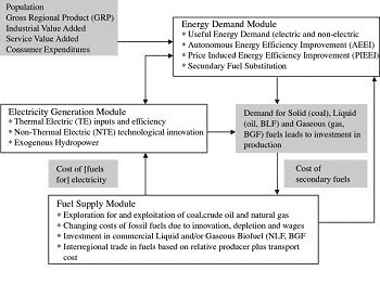
Figure IV-2: Overview of the IMAGE EIS/TIMER model.
|
In the ASF model balancing the supply and demand for energy is achieved ultimately
by adjusting energy prices. Energy prices differ by region to reflect regional
market conditions, and by type of energy to reflect supply constraints, conversion
costs, and the value of the energy to end users. ASF estimates the supply-demand
balance by an iterative search technique to determine supply prices. These supply
prices, which energy producers charge for the fuel at the wellhead or at the
mine, are used to estimate the secondary energy prices in each region. These
secondary prices are based on the supply price for the marginal export region,
the interregional transportation cost, refining and distribution costs, and
regional tax policies. For electricity, the secondary prices reflect the relative
proportions of each fuel used to produce the electricity, the secondary prices
of those fuels, the non-fossil costs of converting the fuels into electricity,
and the conversion efficiency.
The agricultural ASF model estimates the production of major agricultural products,
such as meat, milk, and grain, which is driven by population and gross national
product (GNP) growth. This model is linked with the ASF deforestation model,
which estimates the area of land deforested annually as a function of population
growth and demand for agricultural products.
The ASF GHG emissions model uses outputs of the energy, agricultural, and deforestation
models to estimate GHG emissions in each ASF region. These emissions are estimated
by mapping GHG emission sources to the corresponding emission drivers and changing
them according to changes in these drivers. For example, CH4 emissions from
landfills are mapped to population, while CO2 emissions from cement production
are mapped to GNP.
Finally, the ASF atmospheric model uses GHG emission estimates to calculate
GHG concentrations, and corresponding radiative forcing and temperature effects.
A detailed description of the ASF is provided in the ASF 1990 Report to Congress
(Lashof and Tirpak, 1990), and recent applications of the model are reported
in Pepper et al. (1998) and Sankovski et al. (2000).
IV.3. Integrated Model to Assess the Greenhouse Effect
The Integrated Model to Assess the Greenhouse Effect (IMAGE 2) consists of
three fully linked systems of models:
- The Energy-Industry System (EIS).
- The Terrestrial Environment System (TES).
- The Atmosphere-Ocean System (AOS).
|

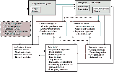
Figure IV-3: The structure of the TES of IMAGE
2 (including links to other modules).
|
Table IV-3: IMAGE
2 regions (see also Table IV-I).
Canada
USA
Latin America (Central and South)
Africa
OECD Europe
Eastern Europe
CIS (former Soviet Union)
Middle East India (including Bangladesh, Bhutan, India, Myanmar, Nepal,
Pakistan, Sri Lanka)
China (including China, Korea (DPR), Kampuchea, Laos, Mongolia, Vietnam)
East Asia South (Indonesia, Republic of Korea, Malaysia, Philippines, Thailand)
Oceania
Japan
|
EIS computes the emissions of GHGs in 13 world regions (Tables IV-1
and IV-3). The energy-related emissions are based on the Targets Image
Energy Regional (TIMER) simulation model (Figure IV-2).
TIMER is a systems dynamics model with investment decisions in energy
efficiency, electricity generation, and energy supply based on anticipated
demand, relative costs or prices, and institutional and informational
delays. The model uses five economic sectors. Technological change and
fuel price dynamics influence energy intensity, fuel substitution, and
the penetration of non-fossil options such as solar electricity and biomass-based
fuels.
The objective of TES is to simulate global land-use and land-cover changes
and their effect on emissions of GHGs and ozone precursors, and on carbon
fluxes between the biosphere and the atmosphere (Figure
IV-3). This subsystem can be used to:
|
- Evaluate the effectiveness of land-use policies to control the build-up
of GHGs.
- Assess the land consequences of large-scale use of biofuels.
- Evaluate the impact of climate change on global ecosystems and agriculture.
- Investigate the effects of population, economic, and technological trends
on changing global land cover.
More detailed information can be obtained by referring to the following web
site: http://sedac.ciesin.org/mva/.
|