IV.6. The Mini Climate Assessment Model
The Mini Climate Assessment Model (MiniCAM) is a small rapidly running Integrated
Assessment Model that estimates global GHG emissions with the ERB model (Edmonds
et al., 1994, 1996a) and the agriculture, forestry and land-use model
(Edmonds et al., 1996b). MiniCAM uses the Wigley and Raper MAGICC (Wigley
and Raper, 1993) model to estimate climate changes, the Hulme et al.
(1995) SCENGEN tool to estimate regional climate changes, and the Manne et
al. (1995) damage functions to examine the impacts of climate change. MiniCAM,
developed by the Global Change Group at Pacific Northwest Laboratory, undergoes
regular enhancements. Recent changes include the addition of an agriculture
land-use module and the capability to estimate emissions of all the Kyoto gases.
At present the model consists of 11 regions (USA, Canada, Western Europe, Japan,
Australia, Eastern Europe and the Former Soviet Union, Centrally Planned Asia,
the Mid-East, Africa, Latin America, and South and East Asia) that provide complete
world coverage (see Table IV-1). A 14-region version
is nearing completion.
MiniCAM uses a straightforward population times labor productivity process
to estimate aggregate labor productivity levels. The resultant estimate of GNP
is corrected for the impact of changes in energy prices using GNP/energy elasticity.
For the scenario exercise, an extended economic activity level process was developed
to allow a clearer understanding of the potential impacts of the new population
scenarios. First, a detailed age breakdown was included so working age populations
could be computed. Second, a labor force participation rate was added to estimate
the labor force, and third an external process was created to estimate the long-term
evolution of the rate of labor productivity increase.
ERB is a partial equilibrium model that uses prices to balance energy supply
and demand for the seven major primary energy categories (coal, oil, gas, nuclear,
hydro, solar, and biomass) in the eleven regions in the model.
The energy demand module initially estimates demands for three categories of
energy services (residential/commercial, industrial, and transportation) as
a function of price and income. Energy services are provided by four secondary
fuels (solids, liquids, gases, and electricity). Demand for the secondary fuels
depends upon their relative costs and the evolution of the end-use technologies,
represented by the improvement in end-use energy efficiency. Demand for primary
fuels is determined by the relative costs of transforming them into the secondary
fuels. Nuclear, solar, and hydro are directly consumed by the electricity sector,
while coal and biomass can be transformed into gas and liquids if the fossil
oil and gas become too expensive or run out. Hydrogen has recently been added
to the model, and it, like refined gas and oil, can be used to generate electricity
or as a secondary fuel for the three final demand sectors.
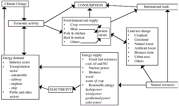
|

Figure IV-5: Structure of the MARIA model of one
region.
|
The energy supply sector provides both renewable (hydro, solar, and biomass)
and non-renewable (coal, oil, gas, and nuclear) resources. The cost of the fossil
resources relates to the resource base by grade, the cost of production (both
technical and environmental), and to historical production capacity. The introduction
of a graded resource base for fossil fuel allows the model to test explicitly
the importance of fossil fuel resource constraints as well as to represent unconventional
fuels such as shale oil and methane hydrates. For unconventional fuels only
small amounts are available at low costs, but large amounts are potentially
available at high cost, or after extensive technology development. Fuel-specific
rates of technical change are available for primary fuel production and conversion,
as are technical change coefficients for each category of electricity production.
Biomass is supplied by the agriculture sector, and provides the link between
the agriculture, forestry, and land-use module and the energy module. The former
module estimates the allocation of land to one of five activities (crops, pasture,
forestry, modern biomass, and other) in each region. This allocation reflects
the relative profitability of each of these uses. Profitability is determined
by the prices for crops, livestock, forest products, and biomass, which reflect
regional demand and supply functions for each product. There are separate technical
change coefficients for crops, livestock/pasture, forestry, and modern biomass
production.
Once the model has reached equilibrium for a period, emissions of GHGs are
computed. For energy, emissions of CO2, CH4 and N2O reflect fossil fuel use
by type of fuel, while agriculture emissions of these gases reflect land-use
change, the use of fertilizer, and the amount and type of livestock produced.
The high global warming gases (chlorofluoro-carbons, hydrochlorofluorocarbons,
hydrofluorocarbons, and perfluorocarbons) are estimated only for each category
and not by their individual components. Sulfur emissions are estimated as a
function of fossil fuel use and reflect sulfur controls, the effectiveness of
which is determined by a Kuznets curve that relates control levels to per capita
income.
The emissions estimates are aggregated to a global level and used as inputs
to MAGICC to produce estimates of GHG concentrations, changes in radiative forcing,
and consequent changes in global mean temperature. The global mean temperature
change is used to drive SCENGEN-derived changes in climate patterns and to produce
estimates of regional change in temperature, precipitation, and cloud cover.
Finally, the regional changes in temperature are used to estimate market and
non-market based damages. Developing region damage functions produce higher
damages than those for developed regions, reflecting the higher vulnerability
of regions with low per capita income.
More detailed information can be obtained by referring to the following web
site: http://sedac.ciesin.org/mva/.
|