|
2.4.5. Gross World Product
|

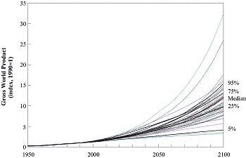
Figure 2-5: Gross world product
- historical development and 193 scenarios, shown as an index (1990
= 1). Data source: UN, 1993a, 1993b; Morita and Lee, 1998.
|
Economic development and growth are fundamental prerequisites to achieve an
increase in living standards. It is thus not surprising that assumptions about
economic development constitute among the most important determinants of emissions
levels in the scenarios. However, economic growth prospects are among the most
uncertain determinants of future emissions. Figure 2-5
shows the future increase in gross world product compared with the historical
experience since 1950. As the differences in base-year data are relatively large,
the gross world product paths are plotted as an index and spliced to historical
data in 1990.
The historical gross world product growth rate has been about 4% per year since
1950; in the scenarios the average annual growth rates to 2100 range from 3.2%
per year to 1.1% per year, with the median value at 2.3% per year. Table
2-3 summarizes the future economic growth rates of the 148 scenarios in
the database that report gross world product for 2100. This translates into
a gross world product level in 2100 that varies from 3.2 (IS92c, Pepper et
al., 1992) to more than 32 (FUND/EMF Modeler's choice, Tol, 1995) times
the 1990 gross world product. The 1990 gross world product was about US$20 trillion
(all values in 1990 US dollars), which translates into a range from more than
US$700 to about US$65 trillion by 2100.
Figure 2-5 also indicates that this full range includes
a few noticeable outliers toward the high and low of future gross world product
development. The rest of the scenarios are grouped much more closely together,
which compresses the range to a factor increase of about 17 to 7 (129 out of
148 scenarios) times compared to 1990. The degree of clustering is discussed
in greater detail in the histograms that follow.
| Table 2-3: Future economic
growth rates for the maximum, minimum, median, and percentiles of the 148
scenarios in the database that report gross world product for 2100 (percent
per year). |
|
| |
1990-2020
|
1990-2050
|
1990-2100
|
|
| Maximum |
3.8
|
3.6
|
3.2
|
| 95% |
3.2
|
2.9
|
2.4
|
| 75% |
2.8
|
2.6
|
2.3
|
| Median |
2.7
|
2.5
|
2.3
|
| 25% |
2.6
|
2.4
|
2.1
|
| 5% |
2.0
|
1.7
|
1.3
|
| Minimum |
1.5
|
1.4
|
1.1
|
|
2.4.6. Gross World Product Histograms
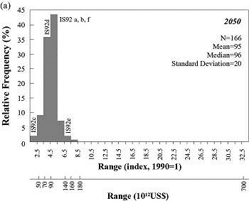
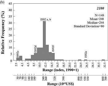
Figures 2-6a and 2-6b
depict the range of gross world product in 2050 and 2100 across all scenarios
in the database9.
The lower horizontal axis shows the factor increase of gross world product compared
with the 1990 value (about US$20 trillion). The second horizontal axis multiplies
the index by the 1990 gross world product to indicate absolute values for each
histogram.
For 2050 most of the scenarios cluster in a rather narrow range around a value
of about US$100 trillion. In total, 166 scenarios were used to derive the histogram
for 2050. This picture changes radically for the year 2100, with a very wide
variation of gross world product values, from about US$700 to US$70 trillion,
and a median of US$250 trillion. As expected, the distribution of emissions
becomes significantly wider as the scenarios extend further into the future.
Most of the distribution is concentrated between about US$320 and US$160 trillion,
with very thin and asymmetric tails. A very strong peak of values lies at around
US$250 trillion, which apparently represents an apparent consensus among modelers
based on an average economic growth rate of about 2.3% per year. The frequency
of the mode is smaller in 2100 than in 2050, which indicates that the scenarios
agree less about the central estimated gross world product (Tol, 1995; Yohe,
1995). For 2050 and 2100 the gross world products for the IS92a and b scenarios
are the same as the median for all scenarios reviewed (Pepper et al.,
1992). 148 different scenarios were used to derive the histogram for the year
2100.

|
| Figure 2-6a: Histogram showing frequency distribution
of gross world product in 2050 for 166 scenarios. The upper horizontal axis
shows indexed gross world product (1990 = 1); the lower axis indicates approximate
absolute values by multiplying the index by the 1990 value (US$20 trillion).
For reference, the gross world products of the IS92 scenarios are indicated.
The frequency distribution associated with scenarios from the literature
does not imply probability of occurrence. |
|

|
| Figure 2-6b: Histogram showing frequency distribution
of gross world product in 2100 for 148 scenarios. The upper horizontal axis
shows indexed gross world product (1990 = 1); the lower axis indicates approximate
absolute values by multiplying the index by the 1990 value (US$20 trillion).
For reference, the gross world products of the IS92 scenarios are indicated.
The frequency distribution associated with scenarios from the literature
does not imply probability of occurrence. |
|