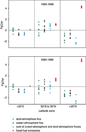
Figure 3.5: Inverse model estimates of fossil fuel CO2 uptake by latitude bands according to eight models using different techniques and sets of atmospheric observations (results summarised by Heimann, 2001). Positive numbers denote fluxes to the atmosphere; negative numbers denote uptake from the atmosphere. The ocean-atmosphere fluxes represent mainly the natural carbon cycle; the land-atmosphere fluxes may be considered as estimates of the uptake of anthropogenic CO2 by the land (with some caveats as discussed in the text). The sum of land-atmosphere and ocean-atmosphere fluxes is shown because it is somewhat better constrained by observations than the separate fluxes, especially for the 1980s when the measurement network was less extensive than it is today. The 1990s are represented by the period 1990 to 1996 only, because when this exercise was carried out the modelling groups did not have access to all of the necessary data for more recent years.

Inverse modelling attempts to resolve regional patterns of CO₂ uptake and release from observed spatial and temporal patterns in atmospheric CO₂ concentrations, sometimes also taking into consideration O₂ and/or ¹³C measurements. The most robust results are for the latitudinal partitioning of sources and sinks between northern and southern mid- to high latitudes and the tropics. The observed annual mean latitudinal gradient of atmospheric CO₂ concentration during the last 20 years is relatively large (about 3 to 4 ppm) compared with current measurement accuracy. It is however not as large as would be predicted from the geographical distribution of fossil fuel burning a fact that suggests the existence of a northern sink for CO₂, as already recognised a decade ago (Keeling et al., 1989; Tans et al., 1990; Enting and Mansbridge, 1991).

The nature of this sink, however, cannot be determined from atmospheric CO₂ concentration measurements alone. It might reflect, at least in part, a natural source-sink pattern of oceanic CO₂ fluxes (Keeling et al., 1989; Broecker and Peng, 1992). This view is supported by the early atmospheric CO₂ data from the 1960s (Bolin and Keeling, 1963) which do not show a clear latitudinal gradient, despite the fact that at that time the fossil emissions were already at least half as large as in the 1990s. Quantitative analysis shows that the Northern Hemisphere sink has not changed much in magnitude since the 1960s (Keeling et al., 1989; Fan et al., 1999). On the other hand, the existing air-sea flux measurements do not support the idea of a large oceanic uptake of CO₂ in the Northern Hemisphere (Tans et al., 1990; Takahashi, 1999). An alternative view, therefore, locates a significant fraction of this Northern Hemisphere sink on land. This view is corroborated, at least for the 1990s, by analyses of the concurrent latitudinal gradients of ¹³C (Ciais et al., 1995a,b) and O₂ (Keeling et al., 1996b).

Results of analyses for the 1980s and 1990 to 1996, carried out by eight modelling groups using different atmospheric transport models, observational data, constraints and mathematical procedures, are summarised in Figure 3.5. Only the most robust findings, i.e., estimates of the mean carbon balance for three latitude bands averaged over the two time periods, are shown. The latitude bands are: �southern extratropics� (>30°S), �tropics� (30°S to 30°N) and �northern extratropics� (>30°N). The carbon balance estimates are broken down into land and ocean compartments within each latitude band (Heimann, 2001).

Although the ranges of the estimates in Figure 3.5 limit the precision of any inference from these analyses, some clear features emerge. The inferred ocean uptake pattern shows the sum of two components: the natural carbon cycle in which CO₂ is outgassed in the tropics and taken up in the extratropics, and the perturbation uptake of anthropogenic CO₂. Separation of these two components cannot be achieved from atmospheric measurements alone.

The estimates for the land, on the other hand, in principle indicate the locations of terrestrial anthropogenic CO₂ uptake (albeit with caveats listed below). For 1980 to 1989, the inverse-model estimates of the land-atmosphere flux are -2.3 to -0.6 PgC/yr in the northern extratropics and -1.0 to +1.5 PgC/yr in the tropics. These estimates imply that anthropogenic CO₂ was taken up both in the northern extratropics and in the tropics (balancing deforestation), as illustrated in Figure 3.6. The estimated land-atmosphere flux in the southern extratropics is estimated as close to zero, which is expected given the small land area involved. Estimates of CO₂ fluxes for the period 1990 to 1996 show a general resemblance to those for the 1980s. For 1990 to 1996, the inverse-model estimates of the land-atmosphere flux are -1.8 to -0.7 PgC/yr in the northern extratropics and -1.3 to +1.1 PgC/yr in the tropics. These results suggest a tendency towards a reduced land-atmosphere flux in the tropics, compared to the 1980s. Such a trend could be produced by reduced deforestation, increased CO₂ uptake or a combination of these.

Inverse modelling studies usually attempt greater spatial resolution of sources and sinks than is presented in this section. However, there are large unresolved differences in longitudinal patterns obtained by inverse modelling, especially in the northern hemisphere and in the tropics (Enting et al., 1995, Law et al., 1996; Fan et al., 1998; Rayner et al., 1999a; Bousquet et al., 1999; Kaminski et al., 1999). These differences may be traced to different approaches and several difficulties in inverse modelling of atmospheric CO₂ (Heimann and Kaminski, 1999):

• The longitudinal variations in CO₂ concentration reflecting net surface sources and sinks are on annual average typically <1 ppm. Resolution of such a small signal (against a background of seasonal variations up to 15 ppm in the Northern Hemisphere) requires high quality atmospheric measurements, measurement protocols and calibration procedures within and between monitoring networks (Keeling et al., 1989; Conway et al., 1994).
• Inverse modelling results depend on the properties of the atmospheric transport models used. The north-south transport of the models can be checked by comparing simulations of the relatively well-known inert anthropogenic tracer SF₆ with measured atmospheric concentrations of this tracer, as recently investigated in the TRANSCOM intercomparison project (Denning et al., 1999). Unfortunately there is no currently measured tracer that can be used to evaluate the models� representation of longitudinal transport. Furthermore, the strong seasonality of the terrestrial CO₂ flux in the Northern Hemisphere together with covarying seasonal variations in atmospheric transport may induce significant mean annual gradients in concentration which do not reflect net annual sources and sinks, but which nevertheless have to be modelled correctly if inverse model calculations are to be reliable (Bolin and Keeling, 1963; Heimann et al., 1986; Keeling et al., 1989; Denning et al., 1995; Law et al., 1996). Even the sign of this so-called �rectifier effect� is uncertain. Some scientists believe that it may be responsible for a part of the apparent Northern Hemisphere uptake of CO₂ implied by inverse modelling results (Taylor, 1989; Taylor and Orr, 2000).
• The spatial partitioning of CO₂ uptake could also be distorted by a few tenths of 1 PgC/yr because the atmospheric concentration gradients also reflect the natural fluxes induced by weathering, transport of carbon by rivers and subsequent outgassing from the ocean (see Figure 3.1) (Sarmiento and Sundquist, 1992; Aumont et al., 2001b). Furthermore, the effects of atmospheric transport of carbon released as CO and CH₄ (especially from incomplete fossil fuel burning, tropical biomass burning, and CH₄ from tropical wetlands) with subsequent oxidation to CO₂ is generally neglected. Their inclusion in the inversion leads to corrections of the latitudinal partitioning of up to 0.1 PgC/yr (Enting and Mansbridge, 1991).
• The distribution of atmospheric CO₂ measurement stations (Figure 3.7) is uneven, and severely underrepresents the continents. This underrepresentation is due in part to the problem of finding continental locations where measurements will not be overwhelmed by local sources and sinks.
• Because of the finite number of monitoring stations, the mathematical inversion problem is highly underdetermined. In principle a multitude of different surface source/sink configurations are compatible with the atmospheric data, within their measurement accuracy. Therefore, in order to extract a meaningful solution, additional information on the sources and sinks has to be introduced into the calculation. Examples of this additional information include maps of air-sea fluxes from observations or ocean models, patterns of terrestrial CO₂ exchanges inferred by terrestrial models, and remote sensing data. Thus, many methodological choices about the use of auxiliary data can influence the outcome of the analysis.

Interannual variability of climate is likely to strongly influence the spatial distribution of CO₂ sources and sinks, so that analyses based on a few years of data are insufficient to establish a long-term trend.

In conclusion, the present atmospheric measurement network, current information on air-sea fluxes and current understanding of vertical atmospheric transport are not sufficient to allow full use of the potential of inverse modelling techniques to infer geographically detailed source-sink distributions of anthropogenic CO₂.

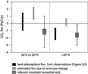
Figure 3.6: Partitioning the 1980s land-atmosphere flux for the tropics and the northern extratropics. The residual terrestrial sink in different latitude bands can be inferred by subtracting the land-use change flux for the 1980s (estimated by modelling studies: Houghton, 1999; Houghton and Hackler, 1999; Houghton et al., 2000; McGuire et al., 2001) from the net land-atmosphere flux as obtained from atmospheric observations by inverse modelling for the same period (Heimann, 2001; results from Figure 3.5). Positive numbers denote fluxes to the atmosphere; negative numbers denote uptake from the atmosphere. This calculation is analogous to the global budget calculation in Table 3.1, but now the model results are broken down geographically and the land-atmosphere fluxes are obtained by inverse modelling. The upper and lower bounds on the residual sink are obtained by pairing opposite extremes of the ranges of values accepted for the two terms in this calculation (for example, by subtracting the bottom of the range of values for land-use change with the top of the range for the land-atmosphere flux). The mid-ranges are obtained by combining similar extremes (for example, subtracting the bottom of the range for land-use change emissions from the bottom of the range land-atmosphere flux).

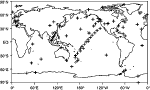
Figure 3.7: The atmospheric CO2 measuring station network as represented by GLOBAL VIEW CO2 (Comparative Atmosphere Data Integration Project -Carbon Dioxide, NOAA/CMDL, http://www.cmdl.noaa.gov/ccg/co2).

IPCC Homepage