Figure 8.8: (a) Vertical structure of the annual-mean, globally averaged temperature (K) from observations and the thirteen models. (b) Latitudinal structure of January temperature at 100 hPa. From Pawson et al. (2000).

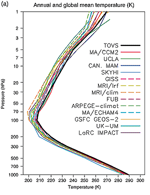
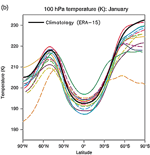
8.5.1.3 Stratospheric climate

Simulation of the stratosphere in coupled climate models is advancing rapidly as the atmospheric components of these models enhance their vertical resolution in the upper part of their domain. Since publication of the SAR, it has become increasingly apparent that comparison between model simulations and observations of the stratosphere play an important role in detection and attribution of climate change (see Chapter 12).

An intercomparison of stratospheric climate simulations (Pawson et al., 2000) shows that all models reproduce to some extent the zonally averaged latitudinal and vertical structure of the observed atmosphere, although several deficiencies are apparent. There is a tendency for the models to show a global mean cold bias at all levels (Figure 8.8a). The latitudinal distribution shows that almost all models are too cold in both hemispheres of the extra-tropical lower stratosphere (Figure 8.8b). There also is a large scatter in the tropical temperatures. Another common model deficiency is in the strengths and locations of the jets. The polar night jets in most models are inclined poleward with height, in noticeable contrast to an equatorward inclination of the observed jet. There is also a differing degree of separation in the models between the winter sub-tropical jet and the polar night jet.
Proper accounting of the role of gravity waves can improve stratospheric modelling. An orographic gravity wave scheme has been shown to improve the cold pole problem. Recent work with non-orographic gravity wave schemes show that waves of non-zero phase speed result in equatorward inclined jet through larger deceleration of westerly winds in polar regions (Manzini and McFarlane, 1998; Medvedev et al., 1998). Nevertheless, all models have shortcomings in their simulations of the present day climate of the stratosphere, which might limit the accuracy of predictions of future climate change (Shindell et al., 1999).

8.5.1.4 Summary

Coupled climate models simulate mean atmospheric fields with reasonable accuracy, with the exception of clouds and some related hydrological processes (in particular those involving upper tropospheric humidity). Since publication of the SAR, the models have continued to simulate most fields reasonably well while relying less on arbitrary flux adjustments. Problems in the simulation of clouds and upper tropospheric humidity, however, remain worrisome because the associated processes account for most of the uncertainty in climate model simulations of anthropogenic change. Incremental improvements in these aspects of model simulation are being made.

8.5.2.1 Developments since the SAR

There have been a number of important developments in the ocean components of climate models since the SAR. Many climate models now being used for climate projections have ocean resolution of order 1 to 2° (Table 8.1), whereas at the time of the SAR most models used in projections had ocean resolution of order 3 to 5° (SAR Tables 5.1 and 6.3). The improved resolution may contribute to better representation of poleward heat transport (Section 8.5.2.2.2), although some key processes are still not resolved (see Sections 8.5.2.3, 8.9.2). Coupled models with even finer resolution are under development at the time of writing, but their computational expense makes their use in climate change projections impractical at present. Advances in the parametrization of sub-grid scale mixing (Chapter 7, Section 7.3.4) have also led to improved heat transports (Section 8.5.2.2.2). Some models have also adopted more advanced parametrizations of the surface mixed layer (Guilyardi and Madec, 1997; Gent et al., 1998; see Chapter 7, Section 7.3.1)

A formal comparison project of a wide range of ocean-climate models has not yet been set up. This is largely because the specification of surface forcing for the ocean, and the long spinup time-scale, make a co-ordinated experimental design more difficult to achieve than for the atmosphere. Nonetheless, a number of smaller, focused projects have provided valuable information about the performance of different model types and the importance of specific processes (Chassignet et al., 1996; Roberts et al., 1996; DYNAMO group 1997). Also, the Ocean Carbon Cycle Intercomparison Project (OCMIP) has compared the ocean circulation in a number of models (Sarmiento et al., 2000; Orr et al., 2001), and some comparisons have been made of the ocean components of coupled models under CMIP (see, e.g., Table 8.2; Jia, 2000)

The observational phase of the World Ocean Circulation Experiment (WOCE) was completed in 1997. Much analysis of the data to date has concentrated on individual sections or regions, and some of this analysis has been used in the assessment of climate models (e.g., Banks, 2000). Some initial attempts to put sections together into a consistent global picture also appear promising (MacDonald, 1998; de las Heras and Schlitzer, 1999). Such a global picture is an important baseline against which models can be tested (Gent et al., 1998; Gordon et al., 2000; see also Chapter 7, Section 7.6).

Table 8.2: Diagnostics of the ocean circulation from a number of coupled model control runs (see Table 8.1 for the specification of models).
MODEL NAME	OVERTURNING ATLANTIC 25N (Sv)	TEMPERATURE CONTRAST ATLANTIC 25N (C)	HEAT TRANSPORT ATLANTIC 25N (PW)	HEAT TRANSPORT PACIFIC 25N (PW)	HEAT TRANSPORT ATLANTIC 30S (PW)	HEAT TRANSPORT INDO-PACIFIC 30S (PW)	ACC TRANSPORT (Sv)	NIÑO 3 SST STD DEV (C)	NIÑO 4 SST STD DEV (C)
ARPEGE/OPA1	16.0	12.4	0.74	0.83	0.20	-0.79	60
ARPEGE/OPA2	12.6	15.9	0.77	0.64	0.33	-0.69	143
CCSR/NIES*	20.8	10.0	0.73	0.32	-0.06	-2.44	200	0.8	0.6
CGCM1*	18.3	9.0	0.72	0.40	0.22	-0.97	62	0.2	0.3
COLA1	16.4	11.0	0.38	0.55	-0.13	-0.48	10
CSIRO Mk 2*	13.0	12.1	0.81	0.43	0.21	-1.31	103
CSM 1.0	24.6	14.0	1.30	0.74	0.54	-1.14	236	0.5	0.5
CSM 1.3	22		1.15	0.8	0.45	-1.10	178
ECHAM1/LSG*	30						100
ECHAM3/LSG*	28.1	9.9	0.76	0.26	0.09	-1.98	112	0.2	0.3
ECHAM4/OPYC3*	22.9	7.3	0.59	0.49	-0.19	-2.31	122	0.8	0.5
GFDL_R15_a*	15.0	9.9	0.59	0.34	0.08	-1.09	70	0.5	0.4
GISS1	18.6	12.3	1.01	0.76	0.37	-0.72	75
GISS2	7.9	21.5	0.56	0.67	0.07	-0.60
GOALS			0.68	0.44	0.05	-1.56	74
HadCM2*	16.8	11.9	0.82	0.34	0.40	-0.93	216
HadCM3	18.1	14.8	1.10	0.51	0.55	-1.25	204	1.1	1.0
IPSL-CM1	11.2	15.2	0.61	0.61	0.27	-0.81	66	0.3	0.2
IPSL-CM2	22.7	11.1	0.90	0.66	0.26	-1.48	164
MRI1*	1.6		-0.29	0.82	-1.00	-1.08	50	0.4	0.7
MRI2*	17.0		0.86	0.78	0.26	-1.21	83	1.9	1.7
NCAR1	35.8	10.3	0.58	0.32	0.80	1.00	79	0.5	0.4
NRL*	3.1		0.43	0.72	-0.10	-0.77	66
DOE PCM	27.2	12.7	1.13	0.77	0.40	-0.73
BMRCa							39	0.4	0.4
COLA2								0.7	0.5
GFDL_R30_c*								0.4	0.6
OBSERVED	19.3a	14.1a	1.15b	0.76c	0.50d	-1.34d	123e	0.7f	0.5f
Positive heat transport values indicate northward transport. An asterisk indicates flux adjusted models. Cells are left blank where particular data items are unavailable. Temperature contrast Atlantic 25°N: The difference between the mean temperatures of the northward flowing surface water and the southward flowing North Atlantic Deep Water at 25°N (Jia 2000). NIÑO3/4 SST Std Dev: standard deviation of the sea surface temperature in the NIÑO3 and NIÑO4 regions of the tropical Pacific. References: a Hall and Bryden, 1982 b Trenberth, 1998a (see Chapter 7, Section 7.6) c Bryden et al., 1991 d MacDonald, 1998 e Whitworth and Petersen, 1985 f Parker et al., 1995

IPCC Homepage