8.5.2.3 Summary
Considerable progress has been made since the SAR in the realism of the ocean
component of climate models. Models now exist which simultaneously maintain
realistic poleward heat transports, surface temperatures and thermocline structure,
and this has been a vital contributor to the improvement in non-flux adjusted
models. However, there are still a number of processes which are poorly resolved
or represented, for example western boundary currents (see Chapter
7, Section 7.3.6), convection (Chapter
7, Section 7.3.2), overflows (Chapter
7, Section 7.3.5), Indonesian through flow, eddies
(including Agulhas eddies which travel long distances and may be hard to treat
by a local parametrization; Chapter 7, Section
7.3.4), Antarctic Bottom Water formation (Chapter 7,
Section 7.3.2) and interior diapycnal mixing (Chapter
7, Section 7.3.3). In many cases, the importance of
these processes in controlling transient climate change has not been evaluated.
Over the next few years there is likely to be a further move to finer resolution
models, and a wider range of model types; these developments are likely to reduce
further some of these uncertainties. Finally, there is still only patchy understanding
of the effects of sub-grid scale parametrizations in the context of coupled
models. Valuable understanding can be gained from sensitivity studies using
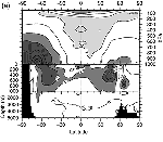
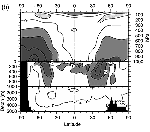
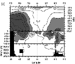
ocean or atmosphere models alone, but Figure 8.9 shows
the inherently coupled nature of the climate system - changes in ocean parametrizations
can have a significant impact throughout the depth of the atmosphere (the reverse
is also true). Further sensitivity studies in the coupled model context will
help to quantify and reduce uncertainty in this area.
|
  
Figure 8.9: Zonal mean air and sea temperature “errors”
in °C (defined here as the difference from the initial model state,
which was derived from observations), for three different coupled models.
The models are all versions of the ARPEGE/OPA model, with T31 atmospheric
resolution, and differ only in the parametrization of lateral mixing used
in the ocean component ((a) lateral diffusion, (b) isopycnal diffusion,
(c) the scheme of Gent and McWilliams (1990)). The different mixing schemes
produce different rates of heat transport between middle and high latitudes,
especially in the Southern Hemisphere. The atmosphere must adjust in order
to radiate the correct amount of heat to space at high latitudes (Chapter
7, Section 7.6 and Section
8.4.1), and this adjustment results in temperature differences at
all levels of the atmosphere. From Guilyardi (1997).
|
8.5.3 Sea Ice Component
While the important role of sea ice in projections of future climate has been
widely recognised (Chapter 7, Section
7.5.2), results of systematic intercomparisons or sensitivity studies of
AOGCM sea-ice components remain very limited. The sea-ice simulations of fifteen
global coupled models contributed to CMIP1 are summarised in Table
8.3. (All these models are also presented in Table
8.1, where the last two columns indicate whether an ice dynamics scheme
is included, and whether the model is flux adjusted.) Sea-ice thermodynamic
formulations of the coupled models are mostly based on simplified schemes: few
employ a multi-layer representation of heat transfer through the ice, while
the rest assume a linear temperature profile. In addition, roughly half of the
models ignore leads and polynyas in the ice although these account for principal
thermodynamic coupling of the atmosphere and ocean. Some models also ignore
the thermodynamic effects of snow on sea ice. Despite the rather mature status
of sea-ice dynamics modelling (e.g., the Sea Ice Model Intercomparison Project
(SIMIP), Lemke et al., 1997), only two of the fifteen models include a physically
based ice dynamics component. Three of the fifteen models allow ice to be advected
with the ocean currents (the so-called ‘free drift’ scheme), and the
remainder assume a motionless ice cover. Overall, this highlights the slow adoption,
within coupled climate models, of advances in stand-alone sea ice and coupled
sea-ice/ocean models (Chapter 7, Section
7.5.2).
| Table 8.3: Coupled model simulations (CMIP1) for
December, January, February (DJF) and June, July, August (JJA) of sea-ice
cover (columns 2 to 5) and snow cover (106 km2) columns
6 and 7). Model names (column 1) are supplemented with ordinal numbers (in
brackets) which refers to the models listed in Table
8.1. The observed sea-ice extent is from Gloersen et al. (1992) and
the climatological observed snow is from Foster and Davy (1988). |
 |
| |
Sea-ice cover (106 km2)

|
Snow cover (106 km2)

|
| |
Northern Hemisphere
|
Southern Hemisphere
|
Northern Hemisphere
|
| Model name |
DJF
(winter)
|
JJA
(summer)
|
JJA
(winter)
|
DJF
(summer)
|
DJF
(winter)
|
JJA
(summer)
|
 |
| ARPEGE/OPA1 (1) |
10.1
|
8.8
|
2.5
|
1.9
|
50.6
|
19.2
|
| BMRCa (3) |
13.7
|
12.0
|
0.0
|
0.0
|
42.4
|
2.2
|
| CCSR/NIES (5) |
13.0
|
9.3
|
16.7
|
8.6
|
46.2
|
12.0
|
| CGCM1 (6) |
8.6
|
7.0
|
12.3
|
8.2
|
47.5
|
13.9
|
| COLA1 (8) |
9.4
|
5.9
|
0.0
|
0.0
|
58.7
|
2.5
|
| CSIRO Mk2 (10) |
14.3
|
14.1
|
14.2
|
13.6
|
48.8
|
18.9
|
| CSM 1.0 (11) |
18.6
|
13.1
|
22.8
|
10.0
|
43.7
|
4.7
|
| ECHAM3/LSG (14) |
12.5
|
10.4
|
11.1
|
7.3
|
35.8
|
9.1
|
| ECHAM4/OPYC3 (15) |
10.5
|
9.1
|
21.0
|
13.4
|
|
|
| GFDL_R15_a (16) |
10.6
|
8.8
|
13.2
|
6.5
|
56.9
|
2.4
|
| GISS1 (19) |
15.3
|
14.6
|
8.7
|
7.1
|
|
|
| GISS2 (20) |
15.7
|
15.2
|
10.9
|
9.5
|
43.2
|
9.3
|
| HadCM2 (22) |
12.0
|
10.1
|
24.7
|
11.8
|
45.0
|
8.2
|
| IPSL-CM1 (24) |
|
|
|
|
44.2
|
11.2
|
| MRI1 (26) |
19.4
|
18.3
|
14.5
|
4.1
|
60.2
|
11.6
|
| NCAR1 (28) |
11.6
|
10.6
|
20.8
|
16.4
|
38.9
|
3.6
|
| |
|
|
|
|
|
|
| Observed |
14.5
|
11.5
|
11.5
|
7.0
|
49.3
|
3.7
|
 |
Table 8.3 provides a comparison of ice extent, defined
as the area enclosed by the ice edge (which is in turn defined as the 0.1 m
thickness contour or the 15% concentration contour, depending on the data provided),
for winter and summer seasons in each hemisphere. The last row of the table
provides an observed estimate based on satellite data (Gloersen et al., 1992)
covering the period 1978 to 1987. It should be noted that assessment of sea-ice
model performance continues to be hampered by observational problems. For the
satellite period (1970s onward) the accuracy of observations of sea-ice concentration
and extent is fair, however observational estimates of sea-ice thickness and
velocity are far from satisfactory.
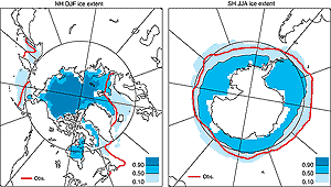
Figure 8.10 provides a visual presentation of the range
in simulated ice extent, and was constructed as follows. For each model listed
in Table 8.3, a 1/0 mask was produced to indicate presence
or absence of ice. The fifteen masks were averaged for each hemisphere and season
and the percentage of models that had sea ice at each grid point was calculated.
|

Figure 8.10: Illustration of the range of sea-ice extent in CMIP1
model simulations listed in Table 8.3: Northern Hemisphere,
DJF (left) and Southern Hemisphere, JJA (right). For each model listed
in Table 8.3, a 1/0 mask is produced to indicate
presence or absence of ice. The fifteen masks were averaged for each hemisphere
and season. The 0.5 contour therefore delineates the region for which
at least half of the models produced sea ice. The 0.1 contour indicates
the region outside of which only 10% of models produced ice, while the
0.9 contour indicates that region inside of which only 10% of models did
not produce ice. The observed boundaries are based on GISST_2.2 (Rayner
et al., 1996) averaged over 1961 to 1990.
|
There is a large range in the ability of models to simulate the position of
the ice edge and its seasonal cycle, particularly in the Southern Hemisphere.
Models that employ flux adjustment tend, on average, to produce smaller ice
extent errors, but there is no obvious connection between fidelity of simulated
ice extent and the inclusion of an ice dynamics scheme. The latter finding probably
reflects the additional impact of errors in the simulated wind field and surface
heat fluxes that offset, to a great extent, any improvements due to including
more realistic parametrizations of the physics of ice motion. In turn this partially
explains the relative slowness in the inclusion of sophisticated sea ice models
with AOGCMs. However, even with quite simple formulations of sea ice, in transient
simulations, some AOGCMs demonstrate ability to realistically reproduce observed
annual trend in the Arctic sea ice extent during several past decades of the
20th century (see Chapter 2, Section
2.2.5.2), which adds some more confidence in the use of AOGCM for future
climate projections (Vinnikov et al., 1999)
|