9.3.4.1 Climate sensititivity

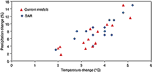
Figure 9.18: Equilibrium climate and hydrological senstitivies from AGCMs coupled to mixed-layer ocean components; blue diamonds from the SAR, red triangles from models in current use (LeTreut and McAvaney, 2000 and Table 9.1).

A variety of feedback processes operate in the climate system (Chapter 7) to determine the response to changes in radiative forcing. The climate sensitivity (see Section 9.2.1) is a broad measure of this response. Ideally, a coupled AOGCM’s climate sensitivity would be obtained by integrating the model to a new climate equilibrium after doubling the CO₂ concentration in the model atmosphere. Since this requires a lengthy integration, climate sensitivities are usually estimated with atmospheric GCMs coupled to mixed-layer upper ocean models, for which the new equilibrium is obtained in decades rather than millennia. Equilibrium climate sensitivities for models in current use are compared with the results reported in the SAR. A related measure, the effective climate sensitivity, is obtained from non-equilibrium transient climate change experiments.

Equilibrium climate sensitivity from AGCMs coupled to mixed-layer upper ocean models
The blue diamonds in Figure 9.18 give the equilibrium climate sensitivity and the associated percentage change in global mean precipitation rate (sometimes termed the hydrological sensitivity) for seventeen equilibrium mixed-layer model calculations documented in Table 6.3 of the SAR (Kattenberg et al., 1996). Table 9.4 gives the average sensitivity of the seventeen models as 3.8°C for temperature and 8.4% for precipitation, with a standard deviation or “inter-model scatter” of 0.78°C and 2.9%, respectively. LeTreut and McAvaney (2000) provide a recent compilation of climate sensitivities for mixed-layer models and this information has been updated in Table 9.1 under the column headed “equilibrium climate sensitivity”. These results, from fifteen models in active use, are represented by the red triangles in Figure 9.18. The associated statistics are given in Table 9.4 where the mean and standard deviation for temperature are 3.5 and 0.92°C, and for precipitation are 6.6 and 3.7%.

According to Table 9.4 and Figure 9.18, the average climate sensitivity, as estimated from AGCMs coupled to mixed-layer ocean models, has decreased slightly from about 3.8 to 3.5°C since the SAR. The inter-model standard deviation has increased and the range has remained essentially the same. The associated hydrological sensitivity has decreased from 8.4 to 6.6% but the inter-model standard deviation has increased. As explained in Section 9.2, these climate sensitivity values are not altered by the lower value for the radiative forcing change for doubled CO₂ discussed in Chapter 6.

Table 9.4: Statistics of climate and hydrological sensitivity for mixed-layer models
Source	No. of models	Temperature (°C)			Precipitation (%)
		Mean	Standard deviation	Range	Mean	Standard deviation	Range
SAR	17	3.8	0.78	1.9 / 5.2	8.4	2.9	3 / 15
Current models	15	3.5	0.92	2.0 / 5.1	6.6	3.7	2 / 15

These results indicate slightly lower average values of sensitivity in models in current use compared with the SAR. Although more recent models attempt to incorporate improvements in our ability to simulate the climate system, these mean results do not in themselves provide a clear indication that modelled climate sensitivity has decreased. In particular, the inter-model scatter has increased slightly, the range of results is not much changed, the differences are not statistically significant, and the reasons for the modest decrease in average sensitivity have not been identified.

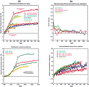
Figure 9.19: (a) AOGCM stabilisation simulations. Upper panel: 1%/yr simulations to stabilisation at and near 2xand 3xCO2. Lower panel: stabilisation experiments starting with historical greenhouse gas forcing up to present day, then going up to 2xor 3xCO2 concentrations following the IS92a scenario, then stabilising in the years 2050 and 2100. (b) Post-stabilisation temperature evolution. Upper panel: Rate of change of the temperature. Lower panel: Temperature evolution after the stabilisation of the greenhouse gas concentration.

Climate sensitivity from AGCMs coupled to full OGCMs
Because of the long time-scales associated with deep ocean equilibration, the direct calculation of coupled model equilibrium temperature change for doubled CO₂ requires an extended simulation and a considerable commitment of computer resources. One such calculation has been performed (Stouffer and Manabe, 1999, Table 9.1); a 4,000 year simulation with stabilisation at 2xCO₂, and a 5,000 year simulation with stabilisation at 4xCO₂. Figure 9.19 displays the temperature for the first 500 years of these simulations (the red curves) together with stabilisation results from other models discussed further below. The calculation shows that: (1) some 15 to 20 centuries are required for the coupled model to attain a new equilibrium after the forcing is stabilised, (2) for the 2xCO₂ case, the temperature change ultimately increases to 4.5°C for the GFDL_R15_a model, which exceeds the 3.9°C value obtained when a mixed-layer ocean is used to estimate the climate sensitivity and, (3) the 4xCO₂ equilibrium temperature change is very nearly twice that of the 2xCO₂ equilibrium temperature change for this model. In this case the mixed-layer value of climate sensitivity is resonably close to the full climate model value. The difference between coupled model and mixed-layer sensitivities for other models is unknown.

Effective climate sensitivity
The term effective climate sensitivity (Murphy, 1995) as defined in Section 9.2.1 is a measure of the strength of the feedbacks at a particular time in a transient experiment. It is a function of climate state and may vary with time. Watterson (2000) calculates the effective climate sensitivity from several experiments with different versions of an AOGCM. The results show considerable variability, particularly near the beginning of the integrations when the temperature change is small. That study nevertheless concludes that the effective climate sensitivity is approximately constant and close to the appropriate equilibrium result. However, estimates of effective climate sensitivity obtained from the HadCM2 model range from about 2.7°C at the time of stabilisation at 2xCO₂ to about 3.8°C after 900 years (Raper et al., 2001a). Senior and Mitchell (2000) implicate time-dependent cloud-feedbacks associated with the slower warming of the Southern Ocean in that model as the cause for this variation in time. The effective climate sensitivity of this climate model is initially considerably smaller than the equilibrium sensitivity obtained with a mixed-layer ocean. As the coupled model integration approaches a new equilibrium, the effective climate sensitivity increases and appears to be approaching the equilibrium climate sensitivity.

If effective climate sensitivity varies with climate state, estimates of climate sensitivity made from a transient simulation may not reflect the ultimate warming the system will undergo. The use of a constant climate sensitivity in simple models will lead to inconsistencies which depend on the value of sensitivity chosen. This feature deserves further study.

Summary
The climate sensitivity is a basic measure of the response of the climate system to a change in forcing. It may be measured in several ways as discussed above. The equilibrium climate sensitivity, that is, the range of the surface air temperature response to a doubling of the atmospheric CO₂ concentration, was estimated to be between 1.5 and 4.5°C in the SAR (Kattenberg et al., 1996). That range still encompasses the estimates from the current models in active use.

IPCC Homepage