2.3.2.2 Characteristics of Stabilization Scenarios
The stabilization scenarios that were estimated based on the above baselines
also have a very wide range, as shown in Figure 2.3.
This wide range is caused by several factors, including differences in emission
time-paths for the stabilization, differences in timing of the stabilization
at 550 ppmv, and different carbon cycle models used to assess the stabilization.
The divergence in reduction time-path has been discussed based on two sets
of popular scenarios. One is a set of IPCC Working Group (WG) I scenarios (Houghton
et al., 1996) which is sometimes referred to as “early action scenarios”
and denoted as “WGI”; the other is a set of scenarios published by
Wigley et al. (1996), sometimes referred to as “delayed action scenarios”
and denoted “WRE”. Chapter 8 explains that
these terms are misleading, since WRE scenarios may not assume early emissions
reductions, but do assume early actions to facilitate such reductions later.
Figure 2.3 compares the 550 ppmv stabilization scenarios
of these two scenario sets with the reviewed scenarios, and it shows that scenarios
reviewed here cover a wider range than that of the WGI and WRE scenarios. While
the RICE and MERGE scenarios show late reduction (WRE type) trajectories, the
CETA, MARIA and MIT scenarios show more severe reduction (WGI type) trajectories.7
A few scenarios, for example ICAM2, show no drastic reduction even in the latter
half of the 21st century. Most of the scenarios have emissions trajectories
that lie in between.
The reduction time-path of emissions is a controversial point, which is closely
related to the intergenerational equity issue. However, no conclusion can be
drawn from such global trajectories, since behind them lies a distribution between
countries and the political, technical, economic, and social acceptability of
this distribution would depend on how the equity concerns are sorted out.
|

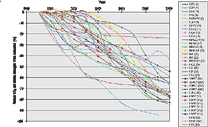
Figure 2.6: Global CO2 emission reduction from baseline
for 550ppmv stabilization scenarios, estimated for each scenario source
as baseline emissions minus emissions in the 550ppmv stabilization scenario
(for legend details see Appendix 2.1).
|
|

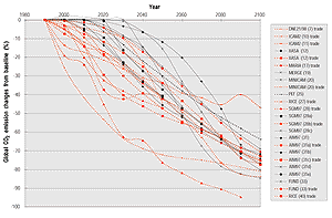
Figure 2.7: Non-OECD CO2 emission reduction for 550ppmv
stabilization, estimated for each scenario source as baseline emissions
minus emissions in the 550ppmv stabilization scenario divided by baseline
emissions. Dotted lines show the scenarios which assume carbon credit
trading between the OECD and developing regions (for legend details see
Appendix 2.1).
|
|

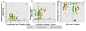
Figure 2.8: Scatter plots to analyze the relationships between
baseline scenario assumptions and mitigation scenario outputs in Energy
Intensity (a), Carbon Intensity (b), and GDP growth (c).
|
Figures 2.6 and 2.7 show energy-related
CO2 reduction at the global and the non-OECD levels, respectively,
which were estimated for each scenario source by subtracting stabilization scenario
emissions (Figure 2.3) from baseline scenario emissions
(Figure 2.2). These figures show that the range
of reduced CO2 emissions for 550ppmv stabilization is also very wide
both at the global and the non-OECD levels. This wide range is apparently caused
by the divergent baseline scenarios shown in Figure
2.2, while other factors such as differences in emission time-path, in timing
of stabilization and in the carbon cycle model used also tend to increase the
range.
Figures 2.6 and 2.7 show the simulation
results of models, assuming that non-OECD countries would participate in mitigation.
The distribution of mitigation among the countries is based on different approaches,
such as the introduction of emission caps, or the assumption of the same rate
of emission reduction for all countries, or global emission trading. The results
show that emission trading may lower the mitigation cost, and could lead to
more mitigation in the non-OECD countries.
The regional allocation of reductions is a controversial and highly political
issue from the equity viewpoint. Mostly, modellers do not explicitly state the
burden-sharing rule. Nevertheless, the emission reduction from baseline by the
non-Annex I countries is a good indicator of when it is assumed that these countries
start sharing the reductions. The data set used in this analysis is limited
in the sense that models have different regional specifications; it was therefore
difficult to obtain a large number of data points to analyze non-Annex I emissions.
As a proxy, emission reduction from the baseline by the non-OECD region is used,
which includes Russia and Eastern Europe. This is shown in Figure
2.7. In part of the AIM, MiniCAM, FUND, and PEF scenarios, introduction
of climate policy in the non-OECD region is assumed not to begin by 2010. Although
Russia and Eastern European countries are included in the Kyoto Protocol, the
models do assume that because of the decreased emissions in these countries
since 1990, actual climate policies would not be needed until 2010. Some scenarios
show that non-OECD regions may not have to significantly reduce emissions before
2030. However, there are still other scenarios that show an opposite picture.
The RICE, MERGE, MIT, and MARIA scenarios show a very steep increase in emission
reduction from baseline levels in the non-OECD region starting very early in
the 21st century.
One of the ways to explain this divergence in reduction time series is to differentiate
the assumptions about trade in these scenarios. Some scenarios assume trade
in emission credits, which are allotted initially to each country or region.
This allows some countries to purchase emission rights from other countries
to minimize the cost of meeting their emission targets. The dotted lines in
Figure 2.7 show the scenarios that assume trade in emission
credits between the Annex I and non-Annex I countries. The scenarios that show
an early reduction of emissions in the non-OECD region are included in the trade
scenarios, and they assume the OECD region would transfer funds to the non-OECD
region via emission credit trading. Most of the other scenarios assume that
the non-OECD region would start to introduce reduction policies after 2010.
With regard to overall mitigation, the range of assumed policies is very wide,
resulting in a wide range of emission reductions. The additional increase in
energy efficiency improvement from the baseline ranges between minus 0.04 and
1.56% per year within the sampled data, while the additional reduction in carbon
intensity from the baseline is between zero and 3.76% per year. Although it
is difficult to identify detailed policy assumptions from the database, the
range of these factors suggests divergent policy options among scenarios. These
policy options are dependent not only on the level of CO2 reduction,
but also on the baseline scenarios that have been used for 550 ppmv stabilization
quantification.
Figure 2.8 (a) shows the relationship between the effects
of efficiency improvement policy in mitigation scenarios and the energy intensity
reduction assumption in baseline scenarios. This figure suggests an inverse
relationship between them. The implication of this is that scenarios in which
there is an assumed adoption of high-efficiency measures in the baseline usually
would have less scope for further introduction of efficiency measures in the
mitigation scenarios, as compared to scenarios that have a lower level of efficiency
improvement in their baseline.8
As a result, the additional reduction of energy intensity in mitigation scenarios
over the base cases would be lower when the assumed energy intensity reduction
is high in the base case, and vice versa. In the case of unanticipated technological
breakthroughs, of course, this relationship may not hold and one could expect
further energy efficiency improvements, even when the baseline has a fair amount
of energy efficiency built into it.
Figure 2.8 (b) shows the relationship between the effects
of decarbonization policies and the carbon intensity reductions assumed in the
baseline scenarios. This figure suggests that baseline scenarios with high carbon
intensity reductions show larger carbon intensity reductions in their mitigation
scenarios, while those with low carbon intensity reductions in the base case
show smaller reductions in carbon intensity in their corresponding stabilization
cases. This is somewhat counterintuitive and difficult to explain simply on
the basis of the results available. One might expect that high carbon intensity
reductions in the base case might “use up” decarbonization potential,
giving rise to lower additional reduction of carbon intensity in mitigation
scenarios. On the other hand, increased investment in low-carbon energy technology
in the base case could increase the resource base of low-carbon energy, thereby
providing more opportunity to reduce CO2 emissions in the stabilization
case. The mitigation potential in this direction depends not only on the technology
but also, and perhaps more, on the economics and social acceptance of the technology.
A closer and more careful analysis of which particular mitigation policies were
assumed in constructing the scenario than was possible on the basis of the available
information, would reveal the underlying reasons for such a pattern.
Finally, Figure 2.8 (c) shows the relationship between
macroeconomic costs9
in the mitigation scenarios and GDP growth assumptions in the baseline scenarios.
No clear relationship is visible, but it can be observed that macroeconomic
costs for the world as a whole are estimated to range between 0% and 3.5% of
GDP in 2100, while a few simple models estimate more increase in the second
half of the 21st century. The GDP loss may or may not be related
to the GDP growth assumptions in baselines. For instance, high baseline economic
growth would lead to higher emissions of GHGs, which would lead to increased
GHG reduction costs compared to the corresponding mitigation scenario for a
low-growth baseline. On the other hand, high economic growth could provide increased
funds for research and development (R&D) of advanced technologies, which
would decrease the cost of GHG reduction. The net cost would depend on the relative
strengths of these effects. Another aspect is that the costs are also dependent
upon the structure of economies, i.e., economies with high fossil fuel dependence,
via either exports or domestic consumption, are likely to experience higher
costs compared with economies with relatively lower fossil fuel dependence.
|