|
What is the range of GHG emissions in the SRES scenarios and how do they
relate to driving forces?
The SRES scenarios cover most of the range of carbon dioxide (CO2 ; see
Figures SPM-2a and SPM-2b), other GHGs, and sulfur emissions found in the
recent literature and SRES scenario database. Their spread is similar to
that of the IS92 scenarios for CO2 emissions from energy and industry as well
as total emissions but represents a much wider range for land-use change. The
six scenario groups cover wide and overlapping emission ranges. The range of
GHG emissions in the scenarios widens over time to capture the long-term uncertainties
reflected in the literature for many of the driving forces, and after 2050 widens
significantly as a result of different socio-economic developments. Table SPM-2b summarizes the emissions across the scenarios in 2020, 2050,
and 2100. Figure SPM-3 shows in greater detail the ranges of total CO2 emissions
for the six scenario groups of scenarios that constitute the four families (the
three scenario families A2, B1, and B2, plus three groups within the A1 family
A1FI, A1T, and A1B).
|
(click to enlarge)
(click to enlarge)
|
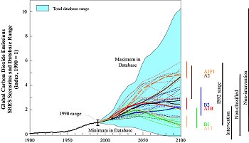
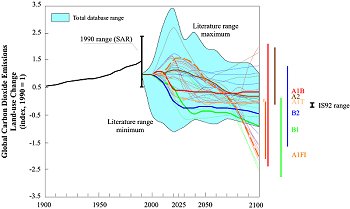
Figure SPM-2: Global CO 2 emissions
related to energy and industry (Figure SPM-2a) and land-use changes
(Figure SPM-2b) from 1900 to 1990, and for the 40 SRES scenarios from
1990 to 2100, shown as an index (1990 = 1). The dashed time-paths depict
individual SRES scenarios and the area shaded in blue the range of scenarios
from the literature as documented in the SRES database. The scenarios
are classified into six scenario groups drawn from the four scenario
families. Six illustrative scenarios are highlighted. The colored vertical
bars indicate the range of emissions in 2100. The four black bars on
the right of Figure SPM-1a indicate the emission ranges in 2100 for
the IS92 scenarios and three ranges of scenarios from the literature,
documented in the SRES database. These three ranges indicate those scenarios
that include some additional climate initiatives (designated as "intervention"
scenarios), those that do not ("non-intervention"), and those that cannot
be assigned to either category ("non-classified"). This classification
is based on a subjective evaluation of the scenarios in the database
and was possible only for energy and industry CO 2 emissions. SAR, Second
Assessment Report.
|
Some SRES scenarios show trend reversals, turning points (i.e., initial
emission increases followed by decreases), and crossovers (i.e., initially emissions
are higher in one scenario, but later emissions are higher in another scenario).
Emission trend reversals (see Figures SPM-2 and SPM-3)
depart from historical emission increases. In most of these cases, the upward
emissions trend due to income growth is more than compensated by productivity
improvements combined with a slowly growing or declining population.
(click to enlarge)
|
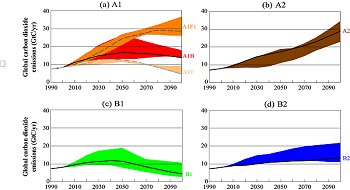
Figure SPM-3: Total global annual
CO2 emissions from all sources (energy, industry, and land-use change)
from 1990 to 2100 (in gigatonnes of carbon (GtC/yr) for the families
and six scenario groups. The 40 SRES scenarios are presented by the
four families (A1, A2, B1, and B2) and six scenario groups: the fossil-intensive
A1FI (comprising the high-coal and high-oil-and-gas scenarios), the
predominantly non-fossil fuel A1T, the balanced A1B in Figure SPM-3a;
A2 in Figure SPM-3b; B1 in Figure SPM-3c, and B2 in Figure SPM-3d. Each
colored emission band shows the range of harmonized and non-harmonized
scenarios within each group. For each of the six scenario groups an
illustrative scenario is provided, including the four illustrative marker
scenarios (A1, A2, B1, B2, solid lines) and two illustrative scenarios
for A1FI and A1T (dashed lines). |
In many SRES scenarios CO2 emissions from loss of forest cover peak after
several decades and then gradually decline 7
(Figure SPM-1b). This pattern is consistent with
scenarios in the literature and can be associated with slowing population growth,
followed by a decline in some scenarios, increasing agricultural productivity,
and increasing scarcity of forest land. These factors allow for a reversal of
the current trend of loss of forest cover in many cases. Emissions decline fastest
in the B1 family. Only in the A2 family do net anthropogenic CO2 emissions from
land use change 2
remain positive through 2100. As was the case for energy-related emissions,
CO2 emissions related to land-use change in the A1 family cover the widest range.
The diversity across these scenarios is amplified through the high economic
growth, increasing the range of alternatives, and through the different modeling
approaches and their treatment of technology.
(click to enlarge)
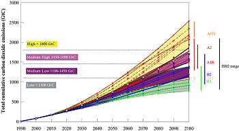
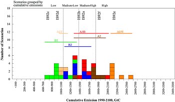
Figure SPM-4: Total global cumulative
CO2 emissions (GtC) from 1990 to 2100 (SPM-4a) and histogram of their
distribution by scenario groups (SPM-4b). No probability of occurrence
should be inferred from the distribution of SRES scenarios or those
in the literature. Both figures show the ranges of cumulative emissions
for the 40 SRES scenarios. Scenarios are also grouped into four cumulative
emissions categories: low, medium-low, medium-high, and high emissions.
Each category contains one illustrative marker scenario plus alternatives
that lead to comparable cumulative emissions, although often through
different driving forces. This categorization can guide comparisons
using either scenarios with different driving forces yet similar emissions,
or scenarios with similar driving forces but different emissions. The
cumulative emissions of the IS92 scenarios are also shown.
(click to enlarge)
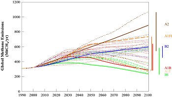
Figure SPM-5: Standardized (to
common 1990 and 2000 values) global annual methane emissions for the
SRES scenarios
(in MtCH4 /yr). The range of emissions by 2100 for the six scenario
groups is indicated to the right. Illustrative (including marker) scenarios
are highlighted.
(click to enlarge)
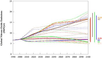
Figure SPM-6: Standardized (to
common 1990 and 2000 values) global annual nitrous oxides emissions
for the SRES scenarios (in MtN/yr). The range of emissions by 2100 for
the six scenario groups is indicated to the right. Illustrative (marker)
scenarios are highlighted.
|
Total cumulative SRES carbon emissions from all sources through 2100 range
from approximately 770 GtC to approximately 2540 GtC. According to the IPCC
Second Assessment Report (SAR), "any eventual stabilised concentration is governed
more by the accumulated anthropogenic CO2 emissions from now until the time
of stabilisation than by the way emissions change over the period." Therefore,
the scenarios are also grouped in the report according to their cumulative emissions.8
(see Figure SPM-4). The SRES scenarios extend the IS92 range toward higher emissions
(SRES maximum of 2538 GtC compared to 2140 GtC for IS92), but not toward lower
emissions. The lower bound for both scenario sets is approximately 770 GtC.
Total anthropogenic methane (CH4) and nitrous oxide (N2O) emissions span
a wide range by the end of the 21st century (see Figures SPM-5
and SPM-6 derived from Figures 5.5
and 5.7). Emissions of these gases in a number
of scenarios begin to decline by 2050. The range of emissions is wider than
in the IS92 scenarios due to the multimodel approach, which leads to a better
treatment of uncertainties and to a wide range of driving forces. These totals
include emissions from land use, energy systems, industry, and waste management.
Methane and nitrous oxide emissions from land use are limited in A1 and
B1 families by slower population growth followed by a decline, and increased
agricultural productivity. After the initial increases, emissions related
to land use peak and decline. In the B2 family, emissions continue to grow,
albeit very slowly. In the A2 family, both high population growth and less rapid
increases in agricultural productivity result in a continuous rapid growth in
those emissions related to land use.
The range of emissions of HFCs in the SRES scenario is generally lower than
in earlier IPCC scenarios. Because of new insights about the availability
of alternatives to HFCs as replacements for substances controlled by the Montreal
Protocol, initially HFC emissions are generally lower than in previous IPCC
scenarios. In the A2 and B2 scenario families HFC emissions increase rapidly
in the second half of the this century, while in the A2 and B2 scenario families
the growth of emissions is significantly slowed down or reversed in that period.
Sulfur emissions in the SRES scenarios are generally below the IS92 range,
because of structural changes in the energy system as well as concerns about
local and regional air pollution. These reflect sulfur control legislation in
Europe, North America, Japan, and (more recently) other parts of Asia and other
developing regions. The timing and impact of these changes and controls vary
across scenarios and regions 9.
After initial increases over the next two to three decades, global sulfur emissions
in the SRES scenarios decrease (see Table SPM-1b),
consistent with the findings of the 1995 IPCC scenario evaluation and recent
peer-reviewed literature.
Similar future GHG emissions can result from very different socio-economic
developments, and similar developments of driving forces can result in different
future emissions. Uncertainties in the future developments of key emission
driving forces create large uncertainties in future emissions, even within the
same socio-economic development paths. Therefore, emissions from each scenario
family overlap substantially with emissions from other scenario families. The
overlap implies that a given level of future emissions can arise from very different
combinations of driving forces. Figures SPM-1, SPM-2,
and SPM-3 show this for CO2 .
Convergence of regional per capita incomes can lead to either high or low
GHG emissions. Tables SPM-1a and SPM-1b
indicate that there are scenarios with high per capita incomes in all regions
that lead to high CO2 emissions (e.g., in the high-growth, fossil fuel intensive
scenario group A1FI). They also indicate that there are scenarios with high
per capita incomes that lead to low emissions (e.g., the A1T scenario group
or the B1 scenario family). This suggests that in some cases other driving forces
may have a greater influence on GHG emissions than income growth.
|