|
9.1.3. Scenario Groups and Four Categories of Cumulative Emissions
|

(click to enlarge)
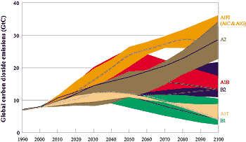
Figure TS-8: Global CO2 emissions
(GtC/yr, standardized) from all sources for the four scenario families
from 1990 to 2100. Scenarios are also presented for the three constituent
groups of the A1 family (fossil-intensive A1FI group, resulting by merging
A1C and A1G as in the SPM, the high non-fossil fuel A1T, and the balanced
A1B) and for the other three families (A2, B1, and B2), forming six
scenario groups altogether. Each colored emission band shows the range
of the scenarios within one group that share common global input assumptions
for population and GDP. The scenarios remaining outside the six groups
adopted alternative interpretations of the four scenario storylines.
|
This comparison of SRES scenario characteristics implies that similar future
emissions can result from very different socio-economic developments, and similar
developments of driving forces can result in different future emissions. Uncertainties
in the future development of key emission driving forces create large uncertainties
in future emissions even within the same socio-economic development paths. Therefore,
emissions from each scenario family overlap substantially with emissions from
other scenario families.
To facilitate comparisons of emissions and their driving forces across the
scenarios, the writing team grouped them into four categories of cumulative
emissions between 1990 and 2100. However, any categorization of scenarios based
on emissions of multiple gases is quite difficult. Figure
TS-8 shows total CO2 emissions from all sources (from Figures
TS-7a and b). The 40 scenarios are shown aggregated into six groups, three
for the A1 family (that result by merging the two fossil-intensive groups A1C
and A1G into one A1FI group as in the SPM). The scenarios that remain outside
the six groups adopted alternative interpretations of the four scenario storylines.
The emission trajectories ("bands") of the scenario groups display different
dynamics, from monotonic increases to non-linear trajectories in which there
is a subsequent decline from a maximum. The dynamics of the individual scenarios
are also different across gasses, sectors, or world regions. This particularly
diminishes the significance of focusing scenario categorization on any given
year, such as 2100. In addition, all gases that contribute to radiative forcing
should be considered, but methods of combining gases such as the use of global
warming potentials (GWPs) are appropriate only for near-term GHG inventories
6
. In light of these difficulties, the classification approach presented here
uses cumulative CO2 emissions between 1990 and 2100. CO2 is the dominant GHG
and cumulative CO2 emissions are expected to be roughly proportional to CO2
radiative forcing over the time scale of a century. According to the IPCC SAR,
"any eventual stabilized concentration is governed more by the accumulated anthropogenic
CO2 emissions from now until the time of stabilization than by the way emissions
change over the period" (Houghton et al., 1996). Therefore, the writing
team also grouped the scenarios according to their cumulative emissions.
|

(click to enlarge)
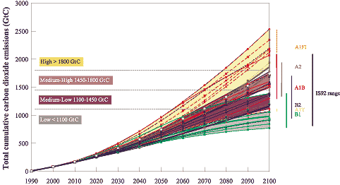
Figure TS-9: Global cumulative
CO2 emissions (GtC, standardized). The ranges of cumulative emissions
for the SRES scenarios are shown. Scenarios are grouped into four categories:
low, medium-low, medium-high, and high emissions. Each category contains
one marker scenario plus alternatives that lead to comparable cumulative
emissions, although often through different driving forces. The ranges
of cumulative emissions of the six SRES scenario groups are shown as
colored vertical bars and the range of the IS92 scenarios as a black
vertical bar.
|
Cumulative SRES carbon emissions through to 2100 range from less than 800 GtC
to more than 2500 GtC with a median of about 1500 GtC. To represent this range,
the scenario classification uses four intervals as follows: less than 1100 GtC
(low), between 1100 and 1450 GtC (medium-low), between 1450 and 1800 GtC (medium-high),
and greater than 1800 GtC (high). Each CO2 interval contains multiple scenarios
and scenarios from more than one family. Each category also includes one of
the four marker scenarios. Figure TS-9 shows how cumulative
carbon emissions from the 40 SRES scenarios fit within the selected emission
intervals (see Chapter 4 for further details). The 40
SRES scenarios extend the IS92 range toward higher emissions (SRES maximum of
2570 GtC compared to 2140 GtC for IS92), but not toward lower emissions. The
lower bound for both scenario sets is just below 800 GtC.
This categorization can guide comparisons using either scenarios with different
driving forces yet similar emissions, or scenarios with similar driving forces
but different emissions. This characteristic of SRES scenarios also has very
important implications for the assessment of climate-change impacts, mitigation,
and adaptation strategies. Two future worlds with fundamentally different characteristic
features, such as the A1B and B2 marker scenarios, also have different cumulative
CO2 emissions and radiative forcing, but very similar CO2 emissions in 2100.
In contrast, scenarios that are in the same category of cumulative emissions
can have fundamentally different driving forces and different CO2 emissions
in 2100, but very similar cumulative emissions and radiative forcing. Presumably,
adverse impacts and effective adaptation measures would vary among the scenarios
from different families that share similar cumulative emissions but have different
demographic, socio-economic, and technological driving forces. This is another
reason for considering the entire range of emissions in future assessments of
climate change.
9.2. Other Greenhouse Gases
Of the GHGs, CO2 is the main contributor to anthropogenic radiative forcing
because of changes in concentrations from pre-industrial times. According to
Houghton et al. (1996) well-mixed GHGs (CO2 ,CH4 ,N2O, and the halocarbons)
induced additional radiative forcing of around 2.5 W/m 2 on a global
and annually averaged basis. CO2 accounted for 60% of the total, which indicates
that the other GHGs are significant as well. Whereas CO2 emissions are by-and-large
attributable to two major sources, energy consumption and land-use change, other
emissions arise from many different sources and a large number of sectors and
applications (e.g. see Table 5-3 in Chapter
5).
The SRES emissions scenarios also have different emissions for other GHGs and
chemically active species such as CO, NOx (nitrogen oxides), and NMVOCs. The
uncertainties that surround the emissions sources of the other GHGs, and the
more complex set of driving forces behind them are considerable and unresolved.
Therefore, the models and approaches employed for the SRES analyses cannot produce
unambiguous and generally approved estimates for different sources and world
regions over a century. Keeping these caveats above in mind, Table
TS-4 (see later) shows the emissions of all relevant direct and indirect
GHGs for the four marker scenarios and, in brackets, the range of the other
scenarios in the same family (or scenario groups for the A1 family). Chapter
5 gives further detail about the full range of GHG emissions across the
SRES scenarios. The emissions of other gases follow dynamic patterns much like
those shown in Figures TS-7 and TS-8
for carbon dioxide emissions. A summary of GHG emissions is given in Chapter
6 and further details in Chapter 5.
|