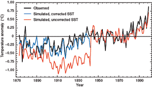
2.2.2.2 Sea surface temperature and ocean air temperature

The analyses of SST described here all estimate the sub-surface bulk temperature, (i.e. the temperature in the first few metres of the ocean) not the skin temperature. Thus the Reynolds and Smith (1994) and Smith et al. (1996) data, which incorporate polar orbiting satellite temperatures, utilise skin temperatures that have been adjusted to estimate bulk SST values through a calibration procedure.

Figure 2.4: Tests of bias adjustments to sea surface temperature (SST) using a climate model (Folland et al., 2001). Black line - annual mean observed land surface air temperature (SAT) anomaly (°C) from a 1946 to 1965 average (Jones, 1994), a period before major anthropogenic warming. Red line � annual averages of four simulations of SAT anomalies using uncorrected SST data, 1872 to 1941, and an average of six simulations for 1941 to 1998. Blue line � average of six simulations of SAT, forced with SST data corrected up to 1941.

Figure 2.5: (a) Annual anomalies of global SST (bars and solid curve) and global night marine air temperature (NMAT, dotted curve), 1861 to 2000, relative to 1961 to 1990 (°C) from UK Met Office analyses (NMAT updated from Parker et al., 1995). Smoothed curves were created using a 21-point binomial filter to give near-decadal averages. Also shown are the equivalent SST anomalies from the SAR � dashed curve. (b) Smoothed annual global SST (°C), 1861 to 2000, relative to 1961 to 1990, from USA National Climate Data Centre, Quayle et al. (1999) (thin dashed line, includes satellite data); USA National Centres for Environmental Prediction, Reynolds and Smith (1994) and Smith et al. (1996) (thin solid line, includes satellite data, to 1999 only), and UK Met Office (Jones et al., 2001) (thick line). (c) UKMO SST and NMAT anomaly time-series from a 1961 to 1990 average for the Northern Hemisphere. (d) As (c) but for the Southern Hemisphere. Both for 1861 to 2000.

Many historical in situ marine data still remain to be digitised and incorporated into the database, to improve coverage and reduce the uncertainties in our estimates of marine climatic variations. A combined physical-empirical method (Folland and Parker, 1995) is used, as in the SAR, to estimate adjustments to ships� SST data obtained up to 1941 to compensate for heat losses from uninsulated (mainly canvas) or partly-insulated (mainly wooden) buckets (see Box 2.2). The corrections are independent of the land-surface air temperature data. Confirmation that these spatially and temporally complex adjustments are quite realistic globally is emerging from simulations of the Jones (1994) land-surface air temperature anomalies using the Hadley Centre atmospheric climate model HadAM3 forced with observed SST and sea-ice extents since 1871, updated from Rayner et al. (1996). Figure 2.4 (Folland et al., 2001) shows simulations of global land-surface air temperature anomalies in model runs forced with SST, with and without bias adjustments to the SST data before 1942. All runs with uncorrected SST (only the average is shown) give too cold a simulation of land-surface air temperature for much of the period before 1941 relative to the 1946 to 1965 base period, with a dramatic increase in 1942. All six individual runs with bias-adjusted SST (only the average is shown) give simulated land air temperatures close to those observed so that internal model variability is small on decadal time-scales compared to the signal being sought. These global results are mostly confirmed by ten similar large regional land-surface air temperature analyses (not shown). Hanawa et al. (2000) have provided independent confirmation of the SST bias corrections around Japan. Therefore, our confidence in the SST data sets has increased. Marine data issues are discussed further in Box 2.2, in Trenberth et al. (1992) and Folland et al. (1993).

Figure 2.5a shows annual values of global SST, using a recently improved UKMO analysis that does not fill regions of missing data (Jones et al., 2001), together with decadally smoothed values of SST from the same analysis. NMAT is also shown. These generally agree well after 1900, but NMAT data are warmer before that time with a slow cooling trend from 1860 not seen in the SSTs, though the minimum around 1910 is seen in both series. The SST analysis from the SAR is also shown. The changes in SST since the SAR are generally fairly small, though the peak warmth in the early 1940s is more evident in the more recent analysis, supported by the NMAT analysis. A contribution to decadally averaged global warmth at that time is likely to have arisen from closely spaced multiple El Niño events centred near 1939 to 1941 and perhaps 1942 to 1944 (Bigg and Inonue, 1992; and Figure 2.29). The NMAT data largely avoid daytime heating of ships� decks (Bottomley et al., 1990; Folland and Parker, 1995). Although NMAT data have been corrected for warm biases in World War II they may still be too warm in the Northern Hemisphere at that time (Figure 2.5c), though there is good agreement in the Southern Hemisphere (Figure 2.5d). The NMAT analysis is based on that in Parker et al. (1995) but differs from that used in the SAR in that it incorporates optimal interpolated data using orthogonal spatial patterns (eigenvectors). This is similar to the technique described by Kaplan et al. (1997, 1998) but with additional allowance for non-stationarity of the data (Parker et al, 1995). Great care is needed in making these reconstructions in a changing climate, as pointed out by Hurrell and Trenberth (1999). This NMAT analysis has been chosen because of the often very sparse data. NMAT confirms the SST trends in the 20th century until 1991 (see also Table 2.1). After 1991, NMAT warmed at a slower rate than SST in parts of the Southern Hemisphere, notably the South Indian and the tropical South Pacific Oceans. Overall, however, the SST data should be regarded as more reliable, though the relative changes in NMAT since 1991 may be partly real (Christy et al., 2001). The similar trends in SST and island air temperature found by Folland et al. (1997) for four regions of the tropical and extra-tropical South Pacific over much of the last century support the generally greater reliability of the SST data.

Figure 2.5b shows three time-series of changes in global SST. The UKMO series (as in Figure 2.5a) does not include polar orbiting satellite data because of possible time-varying biases in them that remain difficult to correct fully (Reynolds, 1993) though the NCEP (National Centers for Environmental Prediction) data (adapted from Smith et al., 1996 and Reynolds and Smith, 1994), starting in 1950, do include satellite data after 1981.

The NCDC series (updated from Quayle et al., 1999) starts in 1880 and includes satellite data to provide nearly complete global coverage. Up to 1981, the Quayle et al series is based on the UKMO series, adjusted by linear regression to match the NCEP series after 1981. It has a truly global coverage based on the optimally interpolated Reynolds and Smith data. The Kaplan et al. (1998) global analysis is not shown because it makes no allowance for non-stationarity (here the existence of global warming) in its optimum interpolation procedures, as noted by Hurrell and Trenberth (1999). The warmest year globally in each SST record was 1998 (UKMO, 0.43°C, NCDC, 0.39°C, and NCEP, 0.34°C, above the 1961 to 1990 average). The latter two analyses are in principle affected by artificially reduced trends in the satellite data (Hurrell and Trenberth, 1999), though the data we show include recent attempts to reduce this. The global SST show mostly similar trends to those of the land-surface air temperature until 1976, but the trend since 1976 is markedly less (Table 2.1). NMAT trends are not calculated from 1861, as they are too unreliable. The difference in trend between global SST and global land air temperature since 1976 does not appear to be significant, but the trend in NMAT (despite any residual data problems) does appear to be less than that in the land air temperature since 1976. Figures 2.5c and d show that NMAT and SST trends remain very similar in the Northern Hemisphere to the end of the record, but diverge rather suddenly in the Southern Hemisphere from about 1991, as mentioned above. The five warmest years in each of the UKMO, NCDC and NCEP SST analyses have occurred after 1986, four of them in the 1990s in the UKMO analysis.

Particularly strong warming has occurred in the extra-tropical North Atlantic since the mid-1980s (approximately 35° to 65°N, 0° to 35°W not shown). This warming appears to be related in part to the warming phase of a multi-decadal fluctuation (Folland et al., 1986, 1999a; Delworth and Mann, 2000; see Section 2.6), perhaps not confined to the North Atlantic (Minobe, 1997; Chao et al., 2000), though global warming is likely to be contributing too. In addition, the cooling in the north-western North Atlantic south of Greenland, reported in the SAR, has ceased. These features were noted by Hansen et al. (1999).

IPCC Homepage