|
Continued from previous page
Estimates of the variability of global mean surface temperature
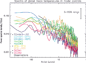
Figure 12.2: Coloured lines: power spectra of global mean temperatures
in the unforced control integrations that are used to provide estimates
of internal climate variability in Figure 12.12.
All series were linearly detrended prior to analysis, and spectra computed
using a standard Tukey window with the window width (maximum lag used in
the estimate) set to one-fifth of the series length, giving each spectral
estimate the same uncertainty range, as shown (see, e.g., Priestley, 1981).
The first 300 years were omitted from ECHAM3-LSG, CGCM1 and CGCM2 models
as potentially trend-contaminated. Solid black line: spectrum of observed
global mean temperatures (Jones et al., 2001) over the period 1861 to 1998
after removing a best-fit linear trend. This estimate is unreliable on inter-decadal
time-scales because of the likely impact of external forcing on the observed
series and the negative bias introduced by the detrending. Dotted black
line: spectrum of observed global mean temperatures after removing an independent
estimate of the externally forced response provided by the ensemble mean
of a coupled model simulation (Stott et al., 2000b, and Figure
12.7c). This estimate will be contaminated by uncertainty in the model-simulated
forced response, together with observation noise and sampling error. However,
unlike the detrending procedure, all of these introduce a positive (upward)
bias in the resulting estimate of the observed spectrum. The dotted line
therefore provides a conservative (high) estimate of observed internal variability
at all frequencies. Asterisks indicate models whose variability is significantly
less than observed variability on 10 to 60 year time-scales after removing
either a best-fit linear trend or an independent estimate of the forced
response from the observed series. Significance is based on an F-test on
the ratio observed/model mean power over this frequency interval and quoted
at the 5% level. Power spectral density (PSD) is defined such that unit-variance
uncorrelated noise would have an expected PSD of unity (see Allen et al.,
2000a, for details). Note that different normalisation conventions can lead
to different values, which appear as a constant offset up or down on the
logarithmic vertical scale used here. Differences between the spectra shown
here and the corresponding figure in Stouffer et al. (2000) shown in Chapter
8, Figure 8.18 are due to the use here
of a longer (1861 to 2000) observational record, as opposed to 1881 to 1991
in Figure 8.18. That figure also shows 2.5
to 97.5% uncertainty ranges, while for consistency with other figures in
this chapter, the 5 to 95% range is displayed here. |
Stouffer et al. (2000) assess variability simulated in
three 1,000-year control simulations (see Figure 12.1).
The models are found to simulate reasonably well the spatial distribution of
variability and the spatial correlation between regional and global mean variability,
although there is more disagreement between models at long time-scales (>50
years) than at short time-scales. None of the long model simulations produces
a secular trend which is comparable to that observed. Chapter
8, Section 8.6.2. assesses model-simulated variability
in detail. Here we assess the aspects that are particularly relevant to climate
change detection. The power spectrum of global mean temperatures simulated by
the most recent coupled climate models (shown in Figure 12.2)
compares reasonably well with that of detrended observations (solid black line)
on interannual to decadal time-scales. However, uncertainty of the spectral
estimates is large and some models are clearly underestimating variability (indicated
by the asterisks). Detailed comparison on inter-decadal time-scales is difficult
because observations are likely to contain a response to external forcings that
will not be entirely removed by a simple linear trend. At the same time, the
detrending procedure itself introduces a negative bias in the observed low-frequency
spectrum.
Both of these problems can be avoided by removing an independent estimate of
the externally forced response from the observations before computing the power
spectrum. This independent estimate is provided by the ensemble mean of a coupled
model simulation of the response to the combination of natural and anthropogenic
forcing (see Figure 12.7c). The resulting spectrum
of observed variability (dotted line in Figure 12.2) will
not be subject to a negative bias because the observed data have not been used
in estimating the forced response. It will, however, be inflated by uncertainty
in the model-simulated forced response and by noise due to observation error
and due to incomplete coverage (particularly the bias towards relatively noisy
Northern Hemisphere land temperatures in the early part of the observed series).
This estimate of the observed spectrum is therefore likely to overestimate power
at all frequencies. Even so, the more variable models display similar variance
on the decadal to inter-decadal time-scales important for detection and attribution.
Estimates of spatial patterns of variability
Several studies have used common empirical orthogonal function (EOF) analysis
to compare the spatial modes of climate variability between different models.
Stouffer et al. (2000) analysed the variability of 5-year means of surface temperature
in 500-year or longer simulations of the three models most commonly used to
estimate internal variability in formal detection studies. The distribution
of the variance between the EOFs was similar between the models and the observations.
HadCM2 tended to overestimate the variability in the main modes, whereas GFDL
and ECHAM3 underestimated the variability of the first mode. The standard deviations
of the dominant modes of variability in the three models differ from observations
by less than a factor of two, and one model (HadCM2) has similar or more variability
than the observations in all leading modes. In general, one would expect to
obtain conservative detection and attribution results when natural variability
is estimated with such a model. One should also expect control simulations to
be less variable than observations because they do not contain externally forced
variability. Hegerl et al. (2000) used common EOFS to compare 50-year June-July-August
(JJA) trends of surface temperature in ECHAM3 and HadCM2. Standard deviation
differences between models were marginally larger on the 50-year time-scale
(less than a factor of 2.5). Comparison with direct observations cannot be made
on this time-scale because the instrumental record is too short.
Variability of the free atmosphere
Gillett et al. (2000a) compared model-simulated variability in the free atmosphere
with that of detrended radiosonde data. They found general agreement except
in the stratosphere, where present climate models tend to underestimate variability
on all time-scales and, in particular, do not reproduce modes of variability
such as the quasi-biennial oscillation (QBO). On decadal time-scales, the model
simulated less variability than observed in some aspects of the vertical patterns
important for the detection of anthropogenic climate change. The discrepancy
is partially resolved by the inclusion of anthropogenic (greenhouse gas, sulphate
and stratospheric ozone) forcing in the model. However, the authors also find
evidence that solar forcing plays a significant role on decadal time-scales,
indicating that this should be taken into account in future detection studies
based on changes in the free atmosphere (see also discussion in Chapter
6 and Section 12.2.3.1 below).
Comparison of model and palaeoclimatic estimates of variability
Comparisons between the variability in palaeo-reconstructions and climate model
data have shown mixed results to date. Barnett et al. (1996) compared the spatial
structure of climate variability of coupled climate models and proxy time-series
for (mostly summer) decadal temperature (Jones et al., 1998). They found that
the model-simulated amplitude of the dominant proxy mode of variation is substantially
less than that estimated from the proxy data. However, choosing the EOFs of
the palaeo-data as the basis for comparison will maximise the variance in the
palaeo-data and not the models, and so bias the model amplitudes downwards.
The neglect of naturally forced climate variability in the models might also
be responsible for part of the discrepancy noted in Barnett et al. (1996) (see
also Jones et al., 1998). The limitations of the temperature reconstructions
(see Chapter 2, Figure 2.21),
including for example the issue of how to relate site-specific palaeo-data to
large-scale variations, may also contribute to this discrepancy. Collins et
al. (2000) compared the standard deviation of large-scale Northern Hemisphere
averages in a model control simulation and in tree-ring-based proxy data for
the last 600 years on decadal time-scales. They found a factor of less than
two difference between model and data if the tree-ring data are calibrated such
that low-frequency variability is better retained than in standard methods (Briffa
et al., 2000). It is likely that at least part of this discrepancy can be resolved
if natural forcings are included in the model simulation. Crowley (2000) found
that 41 to 69% of the variance in decadally smoothed Northern Hemisphere mean
surface temperature reconstructions could be externally forced (using data from
Mann et al. (1998) and Crowley and Lowery (2000)). The residual variability
in the reconstructions, after subtracting estimates of volcanic and solar-forced
signals, showed no significant difference in variability on decadal and multi-decadal
time-scales from three long coupled model control simulations. In summary, while
there is substantial uncertainty in comparisons between long-term palaeo-records
of surface temperature and model estimates of multi-decadal variability, there
is no clear evidence of a serious discrepancy.
Summary
These findings emphasise that there is still considerable uncertainty in the
magnitude of internal climate variability. Various approaches are used in detection
and attribution studies to account for this uncertainty. Some studies use data
from a number of coupled climate model control simulations (Santer et al., 1995;
Hegerl et al., 1996, 1997, North and Stevens, 1998) and choose the most conservative
result. In other studies, the estimate of internal variance is inflated to assess
the sensitivity of detection and attribution results to the level of internal
variance (Santer et al., 1996a, Tett et al., 1999; Stott et al., 2001). Some
authors also augment model-derived estimates of natural variability with estimates
from observations (Hegerl et al., 1996). A method for checking the consistency
between the residual variability in the observations after removal of externally
forced signals (see equation A12.1.1, Appendix
12.1) and the natural internal variability estimated from control simulations
is also available (e.g., Allen and Tett, 1999). Results indicate that, on the
scales considered, there is no evidence for a serious inconsistency between
the variability in models used for optimal fingerprint studies and observations
(Allen and Tett, 1999; Tett et al., 1999; Hegerl et al., 2000, 2001; Stott et
al., 2001). The use of this test and the use of internal variability from the
models with the greatest variability increases confidence in conclusions derived
from optimal detection studies.
|